added 3 characters in body
Source Link
Jens
  • 97.9k
  • 7
  • 215
  • 510

The range of indices for the eigenfunctions in my expansion is determined by the dimensions of the data grid representing the initial values. I.e., the number of basis functions with unknown coefficients is equal to the number of initial data given by the initial wave function. The number of sampling points is determined by the option PlotPoints.

Once I have the fit, the time evolution of the wave consists simply of multiplying each term in the eigenfunction superposition by its time-evolution factor $\exp(-i E_{\mu,\nu})$$\exp(-i t E_{\mu,\nu})$ in dimensionless units (chosen such that the energies are simply $E_{\mu,\nu} = (\mu/L_x)^2+ (\nu/L_y)^2$, where $L_x$ and $L_y$ are the dimensions of the rectangular box.

The range of indices for the eigenfunctions in my expansion is determined by the dimensions of the data grid representing the initial values. I.e., the number basis functions with unknown coefficients is equal to the number of initial data given by the initial wave function. The number of sampling points is determined by the option PlotPoints.

Once I have the fit, the time evolution of the wave consists simply of multiplying each term in the eigenfunction superposition by its time-evolution factor $\exp(-i E_{\mu,\nu})$ in dimensionless units (chosen such that the energies are simply $E_{\mu,\nu} = (\mu/L_x)^2+ (\nu/L_y)^2$, where $L_x$ and $L_y$ are the dimensions of the rectangular box.

The range of indices for the eigenfunctions in my expansion is determined by the dimensions of the data grid representing the initial values. I.e., the number of basis functions with unknown coefficients is equal to the number of initial data given by the initial wave function. The number of sampling points is determined by the option PlotPoints.

Once I have the fit, the time evolution of the wave consists simply of multiplying each term in the eigenfunction superposition by its time-evolution factor $\exp(-i t E_{\mu,\nu})$ in dimensionless units (chosen such that the energies are simply $E_{\mu,\nu} = (\mu/L_x)^2+ (\nu/L_y)^2$, where $L_x$ and $L_y$ are the dimensions of the rectangular box.

added 63 characters in body
Source Link
Jens
  • 97.9k
  • 7
  • 215
  • 510

frames

The majority of the time is spent making the plots. The actual computation is very fast.

The initial condition is converted to a table of initial data on a grid of sampling points that are supposed to be chosen so they don't coincide with the nodal lines of the eigenfunctions $\psi_{\mu,\nu}(x,y)$. Then I ask FindFit to give me a set of expansion coefficients such that a superposition of eigenfunctions reproduces the given initial data in the best possible way. At that stage any conflict with the boundary conditions is removed, because the resulting fit of the initial data will always satisfy them, at the expense of introducing some deviation from the initial function in the domain, if necessary.

The range of indices for the eigenfunctions in my expansion is determined by the dimensions of the data grid representing the initial values. I.e., the number basis functions with unknown coefficients is equal to the number of initial data given by the initial wave function. The number of sampling points is determined by the option PlotPoints.

The majority of the time is spent making the plots. The actual computation is very fast.

The initial condition is converted to a table of initial data on a grid of sampling points that are supposed to be chosen so they don't coincide with the nodal lines of the eigenfunctions $\psi_{\mu,\nu}(x,y)$. Then I ask FindFit to give me a set of expansion coefficients such that a superposition of eigenfunctions reproduces the given initial data in the best possible way. At that stage any conflict with the boundary conditions is removed, because the resulting fit of the initial data will always satisfy them, at the expense of introducing some deviation from the initial function in the domain, if necessary.

frames

The majority of the time is spent making the plots. The actual computation is very fast.

The initial condition is converted to a table of initial data on a grid of sampling points that are supposed to be chosen so they don't coincide with the nodal lines of the eigenfunctions $\psi_{\mu,\nu}(x,y)$. Then I ask FindFit to give me a set of expansion coefficients such that a superposition of eigenfunctions reproduces the given initial data in the best possible way. At that stage any conflict with the boundary conditions is removed, because the resulting fit of the initial data will always satisfy them, at the expense of introducing some deviation from the initial function in the domain, if necessary.

The range of indices for the eigenfunctions in my expansion is determined by the dimensions of the data grid representing the initial values. I.e., the number basis functions with unknown coefficients is equal to the number of initial data given by the initial wave function. The number of sampling points is determined by the option PlotPoints.

Source Link
Jens
  • 97.9k
  • 7
  • 215
  • 510

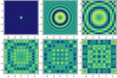
Since there is no spatially or temporally varying potential energy term in the differential equation, it's not efficient to apply NDSolve with the method of lines. The Dirichlet boundary conditions are in principle also inconsistent with the Gaussian initial condition, so one should choose an initial condition that is forced to be zero at the boundary. The narrow initial packet requires a large spatial grid.

To get around this, it's better to expand in the known eigenfunctions of the time-independent Schrödinger equation for the box. Here is a function that does this:

Options[evolve2D] = {PlotPoints -> 10}; 
evolve2D[ψinitial_, {x_, xMin_, xMax_}, {y_, yMin_, yMax_}, t_, 
  OptionsPattern[]] := Module[
  {lx, ly, n, δ, data, ψBox, basis, dim, c, amplitudes},
  lx = xMax - xMin;
  ly = yMax - yMin;
  ψBox[μ_, ν_] := 
   Sin[(μ Pi (x - xMin))/lx] Sin[(ν Pi (y - yMin))/ly];
  n = OptionValue[PlotPoints];
  δ = N[Min[lx, ly]/n];
  data = Table[{x, y, ψinitial}, {x, xMin + δ/2, 
     xMax, δ}, {y, yMin + δ/2, yMax, δ}];
  dim = Most[Dimensions[data]];
  basis = Flatten[Array[c[#, #2] ψBox[#, #2] &, dim]];
  amplitudes = Flatten[Array[c[#, #2] &, dim]];
  Total[basis Flatten[
      Array[Exp[-I t ((#/lx)^2 + (#2/ly)^2)] &, dim]]] /. 
   FindFit[Flatten[data, 1], Total[basis], amplitudes, {x, y}]
  ]

ψ = evolve2D[Exp[-(x^2 + y^2)/.2^2], {x, -5, 5}, {y, -5, 5}, t, 
   PlotPoints -> 30];

frames = Table[
   DensityPlot[Evaluate[Re[ψ]], {x, -5, 5}, {y, -5, 5},
    PlotPoints -> 50, PlotRange -> All, MaxRecursion -> 1, 
    ColorFunction -> "BlueGreenYellow"],
   {t, 0, 12, .1}];

ListAnimate[frames]

The majority of the time is spent making the plots. The actual computation is very fast.

evolve2D is specially written for a rectangular box with Dirichlet boundary conditions, and it uses the known wave functions and energies for that problem.

You give it an arbitrary initial condition, that doesn't even have to be consistent with the boundary conditions. The function will take care of adapting the initial condition to an allowed form automatically. This works by using FindFit:

The initial condition is converted to a table of initial data on a grid of sampling points that are supposed to be chosen so they don't coincide with the nodal lines of the eigenfunctions $\psi_{\mu,\nu}(x,y)$. Then I ask FindFit to give me a set of expansion coefficients such that a superposition of eigenfunctions reproduces the given initial data in the best possible way. At that stage any conflict with the boundary conditions is removed, because the resulting fit of the initial data will always satisfy them, at the expense of introducing some deviation from the initial function in the domain, if necessary.

Once I have the fit, the time evolution of the wave consists simply of multiplying each term in the eigenfunction superposition by its time-evolution factor $\exp(-i E_{\mu,\nu})$ in dimensionless units (chosen such that the energies are simply $E_{\mu,\nu} = (\mu/L_x)^2+ (\nu/L_y)^2$, where $L_x$ and $L_y$ are the dimensions of the rectangular box.