replaced http://mathematica.stackexchange.com/ with https://mathematica.stackexchange.com/
Source Link

I'm so excited now! I might found a solution for a certain type of PDE related problem! The key point is choosing a odd "DifferenceOrder"!

Let's define a auxiliary function first:

mol[n_, o_] := {"MethodOfLines", 
  "SpatialDiscretization" -> {"TensorProductGrid", "MaxPoints" -> n, 
    "MinPoints" -> n, "DifferenceOrder" -> o}}

Then try this:

Tmax = 1; L = 60; gamma = 5000; A = 1;
xmin = 0; xmax = π L; Subscript[ρ, 0] = 1/(1 + A);
mi[x_] := 8 π Subscript[ρ, 0] A L Sin[x/L];

eq1nonstandard = D[m[x, t], t] + v[x, t] D[m[x, t], x] + gamma D[v[x, t], x, x]; 
eq2nonstandard = D[v[x, t], t] + v[x, t] D[v[x, t], x] + 1/2 m[x, t]; 

Vnonstandard = 
 First[v /. NDSolve[{eq1nonstandard == 0, eq2nonstandard == 0, 
     v[x, 0] == 0, m[x, 0] == mi[x], v[xmin, t] == 0, v[xmax, t] == 0,
      m[xmin, t] == 0, m[xmax, t] == mi[xmax]}, {v}, {x, xmin, xmax}, 
     {t, 0, Tmax}, Method -> mol[25, 9]]]

(* The following line allows you to plot the result easily 
   when NDSolve stops at the half-way. *)
{{xl, xr}, {tl, tr}} = Vnonstandard["Domain"];
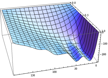
Plot3D[Vnonstandard[x, t], {x, xl, xr}, {t, tl, tr}]
enter image description here

Some observation:

  1. The number of grid points can't be too large, I guess it's because something similar to thisthis happens.

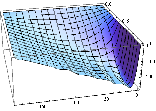
  2. The bigger the "DifferenceOrder" is, the better. This is the result under mol[12, 3]:

enter image description here

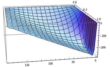
and this is under mol[16, 5]:

enter image description here

  1. Under some "DifferenceOrder", Mathematica can choose suitable number of grid points automatically. For example mol[Automatic, 9].

Nevertheless, I'm not sure why this Method works, this is just a rare victory among my numerous failures when trying to solve the PDE related problem in this site by trial and error.

I'm so excited now! I might found a solution for a certain type of PDE related problem! The key point is choosing a odd "DifferenceOrder"!

Let's define a auxiliary function first:

mol[n_, o_] := {"MethodOfLines", 
  "SpatialDiscretization" -> {"TensorProductGrid", "MaxPoints" -> n, 
    "MinPoints" -> n, "DifferenceOrder" -> o}}

Then try this:

Tmax = 1; L = 60; gamma = 5000; A = 1;
xmin = 0; xmax = π L; Subscript[ρ, 0] = 1/(1 + A);
mi[x_] := 8 π Subscript[ρ, 0] A L Sin[x/L];

eq1nonstandard = D[m[x, t], t] + v[x, t] D[m[x, t], x] + gamma D[v[x, t], x, x]; 
eq2nonstandard = D[v[x, t], t] + v[x, t] D[v[x, t], x] + 1/2 m[x, t]; 

Vnonstandard = 
 First[v /. NDSolve[{eq1nonstandard == 0, eq2nonstandard == 0, 
     v[x, 0] == 0, m[x, 0] == mi[x], v[xmin, t] == 0, v[xmax, t] == 0,
      m[xmin, t] == 0, m[xmax, t] == mi[xmax]}, {v}, {x, xmin, xmax}, 
     {t, 0, Tmax}, Method -> mol[25, 9]]]

(* The following line allows you to plot the result easily 
   when NDSolve stops at the half-way. *)
{{xl, xr}, {tl, tr}} = Vnonstandard["Domain"];
Plot3D[Vnonstandard[x, t], {x, xl, xr}, {t, tl, tr}]

enter image description here

Some observation:

  1. The number of grid points can't be too large, I guess it's because something similar to this happens.

  2. The bigger the "DifferenceOrder" is, the better. This is the result under mol[12, 3]:

enter image description here

and this is under mol[16, 5]:

enter image description here

  1. Under some "DifferenceOrder", Mathematica can choose suitable number of grid points automatically. For example mol[Automatic, 9].

Nevertheless, I'm not sure why this Method works, this is just a rare victory among my numerous failures when trying to solve the PDE related problem in this site by trial and error.

a new observation added.
Source Link
xzczd
  • 68.4k
  • 9
  • 174
  • 489

I'm so excited now! I might found a solution for a certain type of PDE related problem! The key point is choosing a odd "DifferenceOrder"!

Let's define a auxiliary function first:

mol[n_, o_] := {"MethodOfLines", 
  "SpatialDiscretization" -> {"TensorProductGrid", "MaxPoints" -> n, 
    "MinPoints" -> n, "DifferenceOrder" -> o}}

Then try this:

Tmax = 1; L = 60; gamma = 5000; A = 1;
xmin = 0; xmax = π L; Subscript[ρ, 0] = 1/(1 + A);
mi[x_] := 8 π Subscript[ρ, 0] A L Sin[x/L];

eq1nonstandard = D[m[x, t], t] + v[x, t] D[m[x, t], x] + gamma D[v[x, t], x, x]; 
eq2nonstandard = D[v[x, t], t] + v[x, t] D[v[x, t], x] + 1/2 m[x, t]; 

Vnonstandard = 
 First[v /. NDSolve[{eq1nonstandard == 0, eq2nonstandard == 0, 
     v[x, 0] == 0, m[x, 0] == mi[x], v[xmin, t] == 0, v[xmax, t] == 0,
      m[xmin, t] == 0, m[xmax, t] == mi[xmax]}, {v}, {x, xmin, xmax}, 
     {t, 0, Tmax}, Method -> mol[25, 9]]]

(* The following line allows you to plot the result easily 
   when NDSolve stops at the half-way. *)
{{xl, xr}, {tl, tr}} = Vnonstandard["Domain"];
Plot3D[Vnonstandard[x, t], {x, xl, xr}, {t, tl, tr}]

enter image description here

Some observation:

  1. The number of grid points can't be too large, I guess it's because something similar to this happens.

  2. The bigger the "DifferenceOrder" is, the better. This is the result under mol[12, 3]:

enter image description here

and this is under mol[16, 5]:

enter image description here

  1. Under some "DifferenceOrder", Mathematica can choose suitable number of grid points automatically. For example mol[Automatic, 9].

Nevertheless, I'm not sure why this Method works, this is just a rare victory among my numerous failures when trying to solve the PDE related problem in this site by trial and error.

I'm so excited now! I might found a solution for a certain type of PDE related problem! The key point is choosing a odd "DifferenceOrder"!

Let's define a auxiliary function first:

mol[n_, o_] := {"MethodOfLines", 
  "SpatialDiscretization" -> {"TensorProductGrid", "MaxPoints" -> n, 
    "MinPoints" -> n, "DifferenceOrder" -> o}}

Then try this:

Tmax = 1; L = 60; gamma = 5000; A = 1;
xmin = 0; xmax = π L; Subscript[ρ, 0] = 1/(1 + A);
mi[x_] := 8 π Subscript[ρ, 0] A L Sin[x/L];

eq1nonstandard = D[m[x, t], t] + v[x, t] D[m[x, t], x] + gamma D[v[x, t], x, x]; 
eq2nonstandard = D[v[x, t], t] + v[x, t] D[v[x, t], x] + 1/2 m[x, t]; 

Vnonstandard = 
 First[v /. NDSolve[{eq1nonstandard == 0, eq2nonstandard == 0, 
     v[x, 0] == 0, m[x, 0] == mi[x], v[xmin, t] == 0, v[xmax, t] == 0,
      m[xmin, t] == 0, m[xmax, t] == mi[xmax]}, {v}, {x, xmin, xmax}, 
     {t, 0, Tmax}, Method -> mol[25, 9]]]

(* The following line allows you to plot the result easily 
   when NDSolve stops at the half-way. *)
{{xl, xr}, {tl, tr}} = Vnonstandard["Domain"];
Plot3D[Vnonstandard[x, t], {x, xl, xr}, {t, tl, tr}]

enter image description here

Some observation:

  1. The number of grid points can't be too large, I guess it's because something similar to this happens.

  2. The bigger the "DifferenceOrder" is, the better. This is the result under mol[12, 3]:

enter image description here

and this is under mol[16, 5]:

enter image description here

  1. Under some "DifferenceOrder", Mathematica can choose suitable number of grid points automatically. For example mol[Automatic, 9].

Nevertheless, I'm not sure why this Method works, this is just a rare victory among my numerous failures when trying to solve the PDE related problem in this site by trial and error.

add a note.
Source Link
xzczd
  • 68.4k
  • 9
  • 174
  • 489

I'm so excited now! I might found a solution for a certain type of PDE related problem! The key point is choosing a odd "DifferenceOrder"!

Let's define a auxiliary function first:

mol[n_, o_] := {"MethodOfLines", 
  "SpatialDiscretization" -> {"TensorProductGrid", "MaxPoints" -> n, 
    "MinPoints" -> n, "DifferenceOrder" -> o}}

Then try this:

Tmax = 1; L = 60; gamma = 5000; A = 1;
xmin = 0; xmax = π L; Subscript[ρ, 0] = 1/(1 + A);
mi[x_] := 8 π Subscript[ρ, 0] A L Sin[x/L];

eq1nonstandard = D[m[x, t], t] + v[x, t] D[m[x, t], x] + gamma D[v[x, t], x, x]; 
eq2nonstandard = D[v[x, t], t] + v[x, t] D[v[x, t], x] + 1/2 m[x, t]; 

Vnonstandard = 
 First[v /. NDSolve[{eq1nonstandard == 0, eq2nonstandard == 0, 
     v[x, 0] == 0, m[x, 0] == mi[x], v[xmin, t] == 0, v[xmax, t] == 0,
      m[xmin, t] == 0, m[xmax, t] == mi[xmax]}, {v}, {x, xmin, xmax}, 
     {t, 0, Tmax}, Method -> mol[25, 9]]]

(* The following line allows you to plot the result easily 
   when NDSolve stops at the half-way. *)
{{xl, xr}, {tl, tr}} = Vnonstandard["Domain"];
Plot3D[Vnonstandard[x, t], {x, xl, xr}, {t, tl, tr}]

enter image description here

Some observation:

  1. The number of grid points can't be too large, I guess it's because something similar to this happens.

  2. The bigger the "DifferenceOrder" is, the better. This is the result under mol[12, 3]:

enter image description here

and this is under mol[16, 5]:

enter image description here

Nevertheless, I'm not sure why this Method works, this is just a rare victory among my numerous failures when trying to solve the PDE related problem in this site by trial and error.

I'm so excited now! I might found a solution for a certain type of PDE related problem! The key point is choosing a odd "DifferenceOrder"!

Let's define a auxiliary function first:

mol[n_, o_] := {"MethodOfLines", 
  "SpatialDiscretization" -> {"TensorProductGrid", "MaxPoints" -> n, 
    "MinPoints" -> n, "DifferenceOrder" -> o}}

Then try this:

Tmax = 1; L = 60; gamma = 5000; A = 1;
xmin = 0; xmax = π L; Subscript[ρ, 0] = 1/(1 + A);
mi[x_] := 8 π Subscript[ρ, 0] A L Sin[x/L];

eq1nonstandard = D[m[x, t], t] + v[x, t] D[m[x, t], x] + gamma D[v[x, t], x, x]; 
eq2nonstandard = D[v[x, t], t] + v[x, t] D[v[x, t], x] + 1/2 m[x, t]; 

Vnonstandard = 
 First[v /. NDSolve[{eq1nonstandard == 0, eq2nonstandard == 0, 
     v[x, 0] == 0, m[x, 0] == mi[x], v[xmin, t] == 0, v[xmax, t] == 0,
      m[xmin, t] == 0, m[xmax, t] == mi[xmax]}, {v}, {x, xmin, xmax}, 
     {t, 0, Tmax}, Method -> mol[25, 9]]]

(* The following line allows you to plot the result easily 
   when NDSolve stops at the half-way. *)
{{xl, xr}, {tl, tr}} = Vnonstandard["Domain"];
Plot3D[Vnonstandard[x, t], {x, xl, xr}, {t, tl, tr}]

enter image description here

Some observation:

  1. The number of grid points can't be too large, I guess it's because something similar to this happens.

  2. The bigger the "DifferenceOrder" is, the better. This is the result under mol[12, 3]:

enter image description here

and this is under mol[16, 5]:

enter image description here

Nevertheless, I'm not sure why this Method works, this is just a rare victory among my numerous failures when trying to solve the PDE related problem in this site by trial and error.

Source Link
xzczd
  • 68.4k
  • 9
  • 174
  • 489
Loading