Revisions to Line integrals over a path defined by a set of points (rather than an analytic formula)

replaced http://mathematica.stackexchange.com/ with https://mathematica.stackexchange.com/

Source Link

edited Apr 13, 2017 at 12:55

1

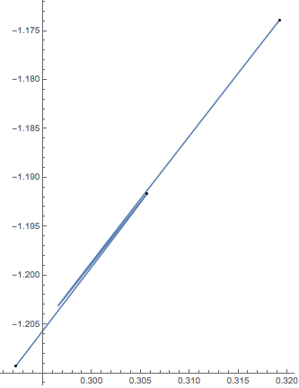
The interpolation overshoots the next point and reverses direction.

ParametricPlot[{line[[1]][tt], line[[2]][tt]}, {tt, 0.2, 0.3}, 
 Epilog -> {Point[points[[All, 1 ;; 2]]]}]

Mathematica graphics

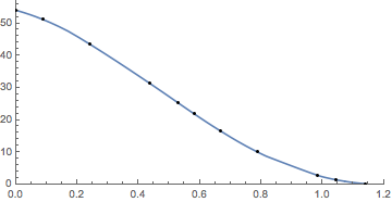
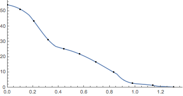
You can reduce the interpolation order to 1 or use a centripetal parametrization parametrizeCurve from J.M.'s answer J.M.'s answer.

parametrizeCurve[pts_List, a : (_?NumericQ) : 1/2] := 
 FoldList[Plus, 0, Normalize[(Norm /@ Differences[pts])^a, Total]] /; 
  MatrixQ[pts, NumericQ]
    
tvals = parametrizeCurve[points];
line = Interpolation[Transpose[{tvals, #}]] & /@ Transpose@points;

s[t_?NumericQ] := 
  NIntegrate[Norm[{line[[1]]'[tt], line[[2]]'[tt]}], 
   Evaluate @ DeleteDuplicates @
     Flatten[{tt, 0, Select[tvals, 0 < # < t &], t}]];

ParametricPlot[
  Evaluate@{s[ss], line[[3]][ss]}, 
  {ss, 0, 1}, 
  PlotRange -> {{0, All}, {0, All}}, 
  AspectRatio -> 1/2, 
  Epilog -> {Point@Table[{s[ss], line[[3]][ss]}, {ss, 0, 1, 0.1}]}
]

Mathematica graphics

Including the interpolation grid points tvals in NIntegrate speeds up the integration. For a really fast implementation use

s = NDSolveValue[{ss'[t] == Norm[{line[[1]]'[t],line[[2]]'[t]}], ss[0]==0}, ss, {t, 0, 1}]

which constructs an InterpolatingFunction for the arc length.

The interpolation overshoots the next point and reverses direction.

ParametricPlot[{line[[1]][tt], line[[2]][tt]}, {tt, 0.2, 0.3}, 
 Epilog -> {Point[points[[All, 1 ;; 2]]]}]

Mathematica graphics

You can reduce the interpolation order to 1 or use a centripetal parametrization parametrizeCurve from J.M.'s answer.

parametrizeCurve[pts_List, a : (_?NumericQ) : 1/2] := 
 FoldList[Plus, 0, Normalize[(Norm /@ Differences[pts])^a, Total]] /; 
  MatrixQ[pts, NumericQ]
    
tvals = parametrizeCurve[points];
line = Interpolation[Transpose[{tvals, #}]] & /@ Transpose@points;

s[t_?NumericQ] := 
  NIntegrate[Norm[{line[[1]]'[tt], line[[2]]'[tt]}], 
   Evaluate @ DeleteDuplicates @
     Flatten[{tt, 0, Select[tvals, 0 < # < t &], t}]];

ParametricPlot[
  Evaluate@{s[ss], line[[3]][ss]}, 
  {ss, 0, 1}, 
  PlotRange -> {{0, All}, {0, All}}, 
  AspectRatio -> 1/2, 
  Epilog -> {Point@Table[{s[ss], line[[3]][ss]}, {ss, 0, 1, 0.1}]}
]

Mathematica graphics

Including the interpolation grid points tvals in NIntegrate speeds up the integration. For a really fast implementation use

s = NDSolveValue[{ss'[t] == Norm[{line[[1]]'[t],line[[2]]'[t]}], ss[0]==0}, ss, {t, 0, 1}]

which constructs an InterpolatingFunction for the arc length.

The interpolation overshoots the next point and reverses direction.

ParametricPlot[{line[[1]][tt], line[[2]][tt]}, {tt, 0.2, 0.3}, 
 Epilog -> {Point[points[[All, 1 ;; 2]]]}]

Mathematica graphics

You can reduce the interpolation order to 1 or use a centripetal parametrization parametrizeCurve from J.M.'s answer.

parametrizeCurve[pts_List, a : (_?NumericQ) : 1/2] := 
 FoldList[Plus, 0, Normalize[(Norm /@ Differences[pts])^a, Total]] /; 
  MatrixQ[pts, NumericQ]
    
tvals = parametrizeCurve[points];
line = Interpolation[Transpose[{tvals, #}]] & /@ Transpose@points;

s[t_?NumericQ] := 
  NIntegrate[Norm[{line[[1]]'[tt], line[[2]]'[tt]}], 
   Evaluate @ DeleteDuplicates @
     Flatten[{tt, 0, Select[tvals, 0 < # < t &], t}]];

ParametricPlot[
  Evaluate@{s[ss], line[[3]][ss]}, 
  {ss, 0, 1}, 
  PlotRange -> {{0, All}, {0, All}}, 
  AspectRatio -> 1/2, 
  Epilog -> {Point@Table[{s[ss], line[[3]][ss]}, {ss, 0, 1, 0.1}]}
]

Mathematica graphics

Including the interpolation grid points tvals in NIntegrate speeds up the integration. For a really fast implementation use

s = NDSolveValue[{ss'[t] == Norm[{line[[1]]'[t],line[[2]]'[t]}], ss[0]==0}, ss, {t, 0, 1}]

which constructs an InterpolatingFunction for the arc length.

Fixed image

Source Link

edited Mar 2, 2015 at 11:13

Michael E2

244.7k
18
351
774

The interpolation overshoots the next point and reverses direction.

ParametricPlot[{line[[1]][tt], line[[2]][tt]}, {tt, 0.2, 0.3}, 
 Epilog -> {Point[points[[All, 1 ;; 2]]]}]

Mathematica graphics

You can reduce the interpolation order to 1 or use a centripetal parametrization parametrizeCurve from J.M.'s answer.

parametrizeCurve[pts_List, a : (_?NumericQ) : 1/2] := 
 FoldList[Plus, 0, Normalize[(Norm /@ Differences[pts])^a, Total]] /; 
  MatrixQ[pts, NumericQ]
    
tvals = parametrizeCurve[points];
line = Interpolation[Transpose[{tvals, #}]] & /@ Transpose@points;

s[t_?NumericQ] := 
  NIntegrate[Norm[{line[[1]]'[tt], line[[2]]'[tt]}], 
   Evaluate @ DeleteDuplicates @
     Flatten[{tt, 0, Select[tvals, 0 < # < t &], t}]];

ParametricPlot[
  Evaluate@{s[ss], line[[3]][ss]}, 
  {ss, 0, 1}, 
  PlotRange -> {{0, All}, {0, All}}, 
  AspectRatio -> 1/2, 
  Epilog -> {Point@Table[{s[ss], line[[3]][ss]}, {ss, 0, 1, 0.1}]}
]

Mathematica graphics

Including the interpolation grid points tvals in NIntegrate speeds up the integration. For a really fast implementation use

s = NDSolveValue[{ss'[t] == Norm[{line[[1]]'[t],line[[2]]'[t]}], ss[0]==0}, ss, {t, 0, 1}]

which constructs an InterpolatingFunction for the arc length.

The interpolation overshoots the next point and reverses direction.

ParametricPlot[{line[[1]][tt], line[[2]][tt]}, {tt, 0.2, 0.3}, 
 Epilog -> {Point[points[[All, 1 ;; 2]]]}]

Mathematica graphics

You can reduce the interpolation order to 1 or use a centripetal parametrization parametrizeCurve from J.M.'s answer.

parametrizeCurve[pts_List, a : (_?NumericQ) : 1/2] := 
 FoldList[Plus, 0, Normalize[(Norm /@ Differences[pts])^a, Total]] /; 
  MatrixQ[pts, NumericQ]
    
tvals = parametrizeCurve[points];
line = Interpolation[Transpose[{tvals, #}]] & /@ Transpose@points;

s[t_?NumericQ] := 
  NIntegrate[Norm[{line[[1]]'[tt], line[[2]]'[tt]}], 
   Evaluate @ DeleteDuplicates @
     Flatten[{tt, 0, Select[tvals, 0 < # < t &], t}]];

ParametricPlot[
  Evaluate@{s[ss], line[[3]][ss]}, 
  {ss, 0, 1}, 
  PlotRange -> {{0, All}, {0, All}}, 
  AspectRatio -> 1/2, 
  Epilog -> {Point@Table[{s[ss], line[[3]][ss]}, {ss, 0, 1, 0.1}]}
]

Mathematica graphics

Including the interpolation grid points tvals in NIntegrate speeds up the integration. For a really fast implementation use

s = NDSolveValue[{ss'[t] == Norm[{line[[1]]'[t],line[[2]]'[t]}], ss[0]==0}, ss, {t, 0, 1}]

which constructs an InterpolatingFunction for the arc length.

The interpolation overshoots the next point and reverses direction.

ParametricPlot[{line[[1]][tt], line[[2]][tt]}, {tt, 0.2, 0.3}, 
 Epilog -> {Point[points[[All, 1 ;; 2]]]}]

Mathematica graphics

You can reduce the interpolation order to 1 or use a centripetal parametrization parametrizeCurve from J.M.'s answer.

parametrizeCurve[pts_List, a : (_?NumericQ) : 1/2] := 
 FoldList[Plus, 0, Normalize[(Norm /@ Differences[pts])^a, Total]] /; 
  MatrixQ[pts, NumericQ]
    
tvals = parametrizeCurve[points];
line = Interpolation[Transpose[{tvals, #}]] & /@ Transpose@points;

s[t_?NumericQ] := 
  NIntegrate[Norm[{line[[1]]'[tt], line[[2]]'[tt]}], 
   Evaluate @ DeleteDuplicates @
     Flatten[{tt, 0, Select[tvals, 0 < # < t &], t}]];

ParametricPlot[
  Evaluate@{s[ss], line[[3]][ss]}, 
  {ss, 0, 1}, 
  PlotRange -> {{0, All}, {0, All}}, 
  AspectRatio -> 1/2, 
  Epilog -> {Point@Table[{s[ss], line[[3]][ss]}, {ss, 0, 1, 0.1}]}
]

Mathematica graphics

Including the interpolation grid points tvals in NIntegrate speeds up the integration. For a really fast implementation use

s = NDSolveValue[{ss'[t] == Norm[{line[[1]]'[t],line[[2]]'[t]}], ss[0]==0}, ss, {t, 0, 1}]

which constructs an InterpolatingFunction for the arc length.

Inserted the derivatives in the appropriate places in the integrand.

Source Link

edit approved Mar 2, 2015 at 8:48

Richard Tasgal

55
4

The interpolation overshoots the next point and reverses direction.

ParametricPlot[{line[[1]][tt], line[[2]][tt]}, {tt, 0.2, 0.3}, 
 Epilog -> {Point[points[[All, 1 ;; 2]]]}]

Mathematica graphics

You can reduce the interpolation order to 1 or use a centripetal parametrization parametrizeCurve from J.M.'s answer.

parametrizeCurve[pts_List, a : (_?NumericQ) : 1/2] := 
 FoldList[Plus, 0, Normalize[(Norm /@ Differences[pts])^a, Total]] /; 
  MatrixQ[pts, NumericQ]
 
    
tvals = parametrizeCurve[points];
line = Interpolation[Transpose[{tvals, #}]] & /@ Transpose@points;

s[t_?NumericQ] := 
  NIntegrate[Norm[{line[[1]][tt]line[[1]]'[tt], line[[2]][tt]line[[2]]'[tt]}], 
   Evaluate @ DeleteDuplicates @
     Flatten[{tt, 0, Select[tvals, 0 < # < t &], t}]];

ParametricPlot[Evaluate@ParametricPlot[
  Evaluate@{s[ss], line[[3]][ss]}, 
  {ss, 0, 1}, 
  PlotRange -> {{0, All}, {0, All}}, 
  AspectRatio -> 1/2, 
  Epilog -> {Point@Table[{s[ss], line[[3]][ss]}, {ss, 0, 1, 0.1}]} 
]

Mathematica graphics

Including the interpolation grid points tvals in NIntegrate speeds up the integration. For a really fast implementation use

s = NDSolveValue[{ss'[t] == Norm[{line[[1]][t]line[[1]]'[t], line[[2]][t]line[[2]]'[t]}], ss[0] == 0ss[0]==0}, ss, {t, 0, 1}]

which constructs an InterpolatingFunction for the arc length.

The interpolation overshoots the next point and reverses direction.

ParametricPlot[{line[[1]][tt], line[[2]][tt]}, {tt, 0.2, 0.3}, 
 Epilog -> {Point[points[[All, 1 ;; 2]]]}]

Mathematica graphics

You can reduce the interpolation order to 1 or use a centripetal parametrization parametrizeCurve from J.M.'s answer.

parametrizeCurve[pts_List, a : (_?NumericQ) : 1/2] := 
 FoldList[Plus, 0, Normalize[(Norm /@ Differences[pts])^a, Total]] /; 
  MatrixQ[pts, NumericQ]
 

tvals = parametrizeCurve[points];
line = Interpolation[Transpose[{tvals, #}]] & /@ Transpose@points;

s[t_?NumericQ] := 
  NIntegrate[Norm[{line[[1]][tt], line[[2]][tt]}], 
   Evaluate @ DeleteDuplicates @
     Flatten[{tt, 0, Select[tvals, 0 < # < t &], t}]];

ParametricPlot[Evaluate@{s[ss], line[[3]][ss]}, {ss, 0, 1}, 
 PlotRange -> {{0, All}, {0, All}}, AspectRatio -> 1/2, 
 Epilog -> {Point@Table[{s[ss], line[[3]][ss]}, {ss, 0, 1, 0.1}]}]

Mathematica graphics

Including the interpolation grid points tvals in NIntegrate speeds up the integration. For a really fast implementation use

s = NDSolveValue[{ss'[t] == Norm[{line[[1]][t], line[[2]][t]}], ss[0] == 0}, ss, {t, 0, 1}]

which constructs an InterpolatingFunction for the arc length.

The interpolation overshoots the next point and reverses direction.

ParametricPlot[{line[[1]][tt], line[[2]][tt]}, {tt, 0.2, 0.3}, 
 Epilog -> {Point[points[[All, 1 ;; 2]]]}]

Mathematica graphics

You can reduce the interpolation order to 1 or use a centripetal parametrization parametrizeCurve from J.M.'s answer.

parametrizeCurve[pts_List, a : (_?NumericQ) : 1/2] := 
 FoldList[Plus, 0, Normalize[(Norm /@ Differences[pts])^a, Total]] /; 
  MatrixQ[pts, NumericQ]
    
tvals = parametrizeCurve[points];
line = Interpolation[Transpose[{tvals, #}]] & /@ Transpose@points;

s[t_?NumericQ] := 
  NIntegrate[Norm[{line[[1]]'[tt], line[[2]]'[tt]}], 
   Evaluate @ DeleteDuplicates @
     Flatten[{tt, 0, Select[tvals, 0 < # < t &], t}]];

ParametricPlot[
  Evaluate@{s[ss], line[[3]][ss]}, 
  {ss, 0, 1}, 
  PlotRange -> {{0, All}, {0, All}}, 
  AspectRatio -> 1/2, 
  Epilog -> {Point@Table[{s[ss], line[[3]][ss]}, {ss, 0, 1, 0.1}]} 
]

Mathematica graphics

Including the interpolation grid points tvals in NIntegrate speeds up the integration. For a really fast implementation use

s = NDSolveValue[{ss'[t] == Norm[{line[[1]]'[t],line[[2]]'[t]}], ss[0]==0}, ss, {t, 0, 1}]

which constructs an InterpolatingFunction for the arc length.

Fixed typos

Source Link

edited Mar 1, 2015 at 19:50

Michael E2

244.7k
18
351
774

Loading

Post Undeleted by Michael E2

occurred Mar 1, 2015 at 16:56

added 1243 characters in body

Source Link

edited Mar 1, 2015 at 16:56

Michael E2

244.7k
18
351
774

Loading

added 49 characters in body

Source Link

edited Mar 1, 2015 at 16:25

Michael E2

244.7k
18
351
774

Loading

Post Deleted by Michael E2

occurred Mar 1, 2015 at 16:20

Source Link

created Mar 1, 2015 at 16:18

Michael E2

244.7k
18
351
774

Loading

Stack Exchange Network

Return to Answer