Revisions to How to connect discrete points and make them become continuous curve?

deleted 21 characters in body

Source Link

edited May 23, 2015 at 3:06

125.5k
11
407
581

One can use the periodicity over $\theta$ and add one periodic copy of the data. In this case FindCurvePath works much better. I also add an interpolation of the result

arrayData = Flatten[Thread@{#, Join[{##2}, {##2} + 2 π]} & @@@ originalData, 1];
curvesPosition = FindCurvePath@arrayData;
{t, θ} = Interpolation@Transpose@{Range[0., 1, 1/(Length@# - 1)], #} & /@ 
      Transpose@arrayData[[#]] & /@ curvesPosition // Transpose;

ParametricPlot[Evaluate@Table[{t[[i]][ξ], θ[[i]][ξ]}, {i, Length@t}], {ξ, 0, 1}, 
 AspectRatio -> 1/GoldenRatio, PlotRange -> {{0, 1}, {0, 4 π}}]

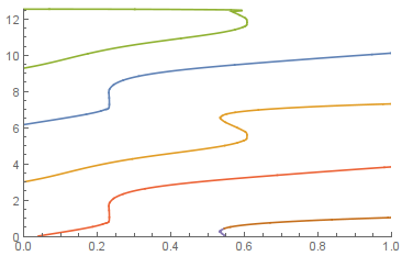
enter image description here plot of data

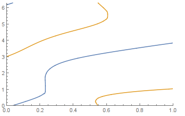
Let's select only full curves and plot them by $\mod 2\pi$$\bmod 2\pi$. Now we explitlyexplicitly see that there are only two branches:

ParametricPlot[{{t[[1]][ξ], Mod[θ[[1]][ξ], 2 π]}, 
  {t[[2]][ξ], Mod[θ[[2]][ξ], 2 π]}}, {ξ, 0, 1}, 
 AspectRatio -> 1/GoldenRatio, PlotRange -> {{0, 1}, {0, 2 π}}]

enter image description here plot with two branches

One can use the periodicity over $\theta$ and add one periodic copy of the data. In this case FindCurvePath works much better. I also add an interpolation of the result

arrayData = Flatten[Thread@{#, Join[{##2}, {##2} + 2 π]} & @@@ originalData, 1];
curvesPosition = FindCurvePath@arrayData;
{t, θ} = Interpolation@Transpose@{Range[0., 1, 1/(Length@# - 1)], #} & /@ 
      Transpose@arrayData[[#]] & /@ curvesPosition // Transpose;

ParametricPlot[Evaluate@Table[{t[[i]][ξ], θ[[i]][ξ]}, {i, Length@t}], {ξ, 0, 1}, 
 AspectRatio -> 1/GoldenRatio, PlotRange -> {{0, 1}, {0, 4 π}}]

enter image description here

Let's select only full curves and plot them by $\mod 2\pi$. Now we explitly see that there are only two branches:

ParametricPlot[{{t[[1]][ξ], Mod[θ[[1]][ξ], 2 π]}, 
  {t[[2]][ξ], Mod[θ[[2]][ξ], 2 π]}}, {ξ, 0, 1}, 
 AspectRatio -> 1/GoldenRatio, PlotRange -> {{0, 1}, {0, 2 π}}]

enter image description here

One can use the periodicity over $\theta$ and add one periodic copy of the data. In this case FindCurvePath works much better. I also add an interpolation of the result

arrayData = Flatten[Thread@{#, Join[{##2}, {##2} + 2 π]} & @@@ originalData, 1];
curvesPosition = FindCurvePath@arrayData;
{t, θ} = Interpolation@Transpose@{Range[0., 1, 1/(Length@# - 1)], #} & /@ 
      Transpose@arrayData[[#]] & /@ curvesPosition // Transpose;

ParametricPlot[Evaluate@Table[{t[[i]][ξ], θ[[i]][ξ]}, {i, Length@t}], {ξ, 0, 1}, 
 AspectRatio -> 1/GoldenRatio, PlotRange -> {{0, 1}, {0, 4 π}}]

plot of data

Let's select only full curves and plot them by $\bmod 2\pi$. Now we explicitly see that there are only two branches:

ParametricPlot[{{t[[1]][ξ], Mod[θ[[1]][ξ], 2 π]}, 
  {t[[2]][ξ], Mod[θ[[2]][ξ], 2 π]}}, {ξ, 0, 1}, 
 AspectRatio -> 1/GoldenRatio, PlotRange -> {{0, 1}, {0, 2 π}}]

plot with two branches

edited body

Source Link

edited Jan 12, 2015 at 14:58

ybeltukov

43.9k
5
109
215

One can use the periodicity over $\theta$ and add one periodic copy of the data. In this case FindCurvePath works much better. I also add an interpolation of the result

arrayData = Flatten[Thread@{#, Join[{##2}, {##2} + 2 π]} & @@@ originalData, 1];
curvesPosition = FindCurvePath@arrayData;
{τt, θ} = Interpolation@Transpose@{Range[0., 1, 1/(Length@# - 1)], #} & /@ 
      Transpose@arrayData[[#]] & /@ curvesPosition // Transpose;

ParametricPlot[Evaluate@Table[{τ[[i]][ξ]t[[i]][ξ], θ[[i]][ξ]}, {i, Length@τLength@t}], {ξ, 0, 1}, 
 AspectRatio -> 1/GoldenRatio, PlotRange -> {{0, 1}, {0, 24 π}}]

enter image description here

Let's select only full curves and plot them by $\mod 2\pi$. Now we explitly see that there are only two branches:

ParametricPlot[{{τ[[1]][ξ]t[[1]][ξ], Mod[θ[[1]][ξ], 2 π]}, 
  {τ[[2]][ξ]t[[2]][ξ], Mod[θ[[2]][ξ], 2 π]}}, {ξ, 0, 1}, 
 AspectRatio -> 1/GoldenRatio, PlotRange -> {{0, 1}, {0, 2 π}}]

enter image description here

One can use the periodicity over $\theta$ and add one periodic copy of the data. In this case FindCurvePath works much better. I also add an interpolation of the result

arrayData = Flatten[Thread@{#, Join[{##2}, {##2} + 2 π]} & @@@ originalData, 1];
curvesPosition = FindCurvePath@arrayData;
{τ, θ} = Interpolation@Transpose@{Range[0., 1, 1/(Length@# - 1)], #} & /@ 
      Transpose@arrayData[[#]] & /@ curvesPosition // Transpose;

ParametricPlot[Evaluate@Table[{τ[[i]][ξ], θ[[i]][ξ]}, {i, Length@τ}], {ξ, 0, 1}, 
 AspectRatio -> 1/GoldenRatio, PlotRange -> {{0, 1}, {0, 2 π}}]

enter image description here

Let's select only full curves and plot them by $\mod 2\pi$. Now we explitly see that there are only two branches:

ParametricPlot[{{τ[[1]][ξ], Mod[θ[[1]][ξ], 2 π]}, 
  {τ[[2]][ξ], Mod[θ[[2]][ξ], 2 π]}}, {ξ, 0, 1}, 
 AspectRatio -> 1/GoldenRatio, PlotRange -> {{0, 1}, {0, 2 π}}]

enter image description here

One can use the periodicity over $\theta$ and add one periodic copy of the data. In this case FindCurvePath works much better. I also add an interpolation of the result

arrayData = Flatten[Thread@{#, Join[{##2}, {##2} + 2 π]} & @@@ originalData, 1];
curvesPosition = FindCurvePath@arrayData;
{t, θ} = Interpolation@Transpose@{Range[0., 1, 1/(Length@# - 1)], #} & /@ 
      Transpose@arrayData[[#]] & /@ curvesPosition // Transpose;

ParametricPlot[Evaluate@Table[{t[[i]][ξ], θ[[i]][ξ]}, {i, Length@t}], {ξ, 0, 1}, 
 AspectRatio -> 1/GoldenRatio, PlotRange -> {{0, 1}, {0, 4 π}}]

enter image description here

Let's select only full curves and plot them by $\mod 2\pi$. Now we explitly see that there are only two branches:

ParametricPlot[{{t[[1]][ξ], Mod[θ[[1]][ξ], 2 π]}, 
  {t[[2]][ξ], Mod[θ[[2]][ξ], 2 π]}}, {ξ, 0, 1}, 
 AspectRatio -> 1/GoldenRatio, PlotRange -> {{0, 1}, {0, 2 π}}]

enter image description here

Source Link

created Jan 12, 2015 at 14:51

ybeltukov

43.9k
5
109
215

One can use the periodicity over $\theta$ and add one periodic copy of the data. In this case FindCurvePath works much better. I also add an interpolation of the result

arrayData = Flatten[Thread@{#, Join[{##2}, {##2} + 2 π]} & @@@ originalData, 1];
curvesPosition = FindCurvePath@arrayData;
{τ, θ} = Interpolation@Transpose@{Range[0., 1, 1/(Length@# - 1)], #} & /@ 
      Transpose@arrayData[[#]] & /@ curvesPosition // Transpose;

ParametricPlot[Evaluate@Table[{τ[[i]][ξ], θ[[i]][ξ]}, {i, Length@τ}], {ξ, 0, 1}, 
 AspectRatio -> 1/GoldenRatio, PlotRange -> {{0, 1}, {0, 2 π}}]

enter image description here

Let's select only full curves and plot them by $\mod 2\pi$. Now we explitly see that there are only two branches:

ParametricPlot[{{τ[[1]][ξ], Mod[θ[[1]][ξ], 2 π]}, 
  {τ[[2]][ξ], Mod[θ[[2]][ξ], 2 π]}}, {ξ, 0, 1}, 
 AspectRatio -> 1/GoldenRatio, PlotRange -> {{0, 1}, {0, 2 π}}]

enter image description here

Stack Exchange Network

Return to Answer