added 135 characters in body
Source Link
rhermans
  • 37.4k
  • 4
  • 61
  • 152

Your data:

data = {{0.067, 0.423}, {0.30, 0.408}, {0.60, 0.433}, {0.25, 0.3512}, {0.37, 0.4602}, {0.44, 0.413}, {0.60, 0.390}, {0.73, 0.437}, {0.8, 0.47}};
errors = {0.055, 0.0552, 0.0662, 0.0583, 0.0378, 0.080, 0.063, 0.072, 0.08};

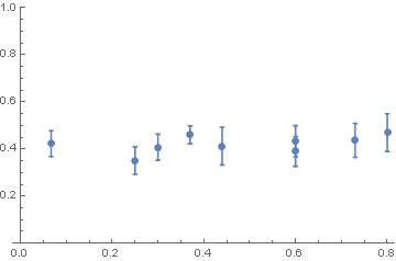
ErrorListPlot[Transpose[{data, ErrorBar /@ errors}], PlotRange -> {0, 1}]

Mathematica graphics

Assume that the errors are distributed Normally with standard deviation given by your errors. Then we can define

diffErr[y1_, s1_, x1_, y2_, s2_, x2_] := Block[{distr, slope, error},
  distr = 
   TransformedDistribution[(v - u)/(
    x2 - x1), {u \[Distributed] NormalDistribution[y1, s1], 
     v \[Distributed] NormalDistribution[y2, s2]}];
  slope = Mean[distr];
  error = StandardDeviation[distr];
  {slope, error}
  ]

That is the calculation of the slope, provided the vertical values are normally distributed with StdDev given by your errors.

And now the slopes between points ie the numerical derivative isderivatives are then

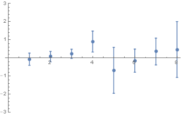
slopes=Table[diffErr[data[[i, 2]], errors[[i]], data[[i, 1]],  data[[i + 1, 2]], errors[[i + 1]], data[[i + 1, 1]]], {i, Length[data] - 1}]
{{-0.0643777, 0.334435}, {0.0833333, 0.287315}, {0.233714, 0.252034}, {0.908333, 0.579016}, {-0.674286, 1.26401}, {-0.14375, 0.636427}, {0.361538, 0.735933}, {0.471429, 1.53756}}
ErrorListPlot[slopes, PlotRange -> {-3, 3}]

Mathematica graphics

Your data:

data = {{0.067, 0.423}, {0.30, 0.408}, {0.60, 0.433}, {0.25, 0.3512}, {0.37, 0.4602}, {0.44, 0.413}, {0.60, 0.390}, {0.73, 0.437}, {0.8, 0.47}};
errors = {0.055, 0.0552, 0.0662, 0.0583, 0.0378, 0.080, 0.063, 0.072, 0.08};

ErrorListPlot[Transpose[{data, ErrorBar /@ errors}], PlotRange -> {0, 1}]

Mathematica graphics

Assume that the errors are distributed Normally with standard deviation given by your errors. Then we can define

diffErr[y1_, s1_, x1_, y2_, s2_, x2_] := Block[{distr, slope, error},
  distr = 
   TransformedDistribution[(v - u)/(
    x2 - x1), {u \[Distributed] NormalDistribution[y1, s1], 
     v \[Distributed] NormalDistribution[y2, s2]}];
  slope = Mean[distr];
  error = StandardDeviation[distr];
  {slope, error}
  ]

And the slopes between points ie the numerical derivative is then

slopes=Table[diffErr[data[[i, 2]], errors[[i]], data[[i, 1]],  data[[i + 1, 2]], errors[[i + 1]], data[[i + 1, 1]]], {i, Length[data] - 1}]
{{-0.0643777, 0.334435}, {0.0833333, 0.287315}, {0.233714, 0.252034}, {0.908333, 0.579016}, {-0.674286, 1.26401}, {-0.14375, 0.636427}, {0.361538, 0.735933}, {0.471429, 1.53756}}
ErrorListPlot[slopes, PlotRange -> {-3, 3}]
Mathematica graphics

Your data:

data = {{0.067, 0.423}, {0.30, 0.408}, {0.60, 0.433}, {0.25, 0.3512}, {0.37, 0.4602}, {0.44, 0.413}, {0.60, 0.390}, {0.73, 0.437}, {0.8, 0.47}};
errors = {0.055, 0.0552, 0.0662, 0.0583, 0.0378, 0.080, 0.063, 0.072, 0.08};

ErrorListPlot[Transpose[{data, ErrorBar /@ errors}], PlotRange -> {0, 1}]

Mathematica graphics

Assume that the errors are distributed Normally with standard deviation given by your errors. Then we can define

diffErr[y1_, s1_, x1_, y2_, s2_, x2_] := Block[{distr, slope, error},
  distr = 
   TransformedDistribution[(v - u)/(
    x2 - x1), {u \[Distributed] NormalDistribution[y1, s1], 
     v \[Distributed] NormalDistribution[y2, s2]}];
  slope = Mean[distr];
  error = StandardDeviation[distr];
  {slope, error}
  ]

That is the calculation of the slope, provided the vertical values are normally distributed with StdDev given by your errors.

And now the slopes between points ie the numerical derivatives are then

slopes=Table[diffErr[data[[i, 2]], errors[[i]], data[[i, 1]],  data[[i + 1, 2]], errors[[i + 1]], data[[i + 1, 1]]], {i, Length[data] - 1}]
{{-0.0643777, 0.334435}, {0.0833333, 0.287315}, {0.233714, 0.252034}, {0.908333, 0.579016}, {-0.674286, 1.26401}, {-0.14375, 0.636427}, {0.361538, 0.735933}, {0.471429, 1.53756}}
ErrorListPlot[slopes, PlotRange -> {-3, 3}]

Mathematica graphics

Source Link
rhermans
  • 37.4k
  • 4
  • 61
  • 152

Your data:

data = {{0.067, 0.423}, {0.30, 0.408}, {0.60, 0.433}, {0.25, 0.3512}, {0.37, 0.4602}, {0.44, 0.413}, {0.60, 0.390}, {0.73, 0.437}, {0.8, 0.47}};
errors = {0.055, 0.0552, 0.0662, 0.0583, 0.0378, 0.080, 0.063, 0.072, 0.08};

ErrorListPlot[Transpose[{data, ErrorBar /@ errors}], PlotRange -> {0, 1}]

Mathematica graphics

Assume that the errors are distributed Normally with standard deviation given by your errors. Then we can define

diffErr[y1_, s1_, x1_, y2_, s2_, x2_] := Block[{distr, slope, error},
  distr = 
   TransformedDistribution[(v - u)/(
    x2 - x1), {u \[Distributed] NormalDistribution[y1, s1], 
     v \[Distributed] NormalDistribution[y2, s2]}];
  slope = Mean[distr];
  error = StandardDeviation[distr];
  {slope, error}
  ]

And the slopes between points ie the numerical derivative is then

slopes=Table[diffErr[data[[i, 2]], errors[[i]], data[[i, 1]],  data[[i + 1, 2]], errors[[i + 1]], data[[i + 1, 1]]], {i, Length[data] - 1}]
{{-0.0643777, 0.334435}, {0.0833333, 0.287315}, {0.233714, 0.252034}, {0.908333, 0.579016}, {-0.674286, 1.26401}, {-0.14375, 0.636427}, {0.361538, 0.735933}, {0.471429, 1.53756}}
ErrorListPlot[slopes, PlotRange -> {-3, 3}]

Mathematica graphics