edited body
Source Link
george2079
  • 39.1k
  • 1
  • 44
  • 111

Here is a case where you should take a close look at the magnituremagnitude of your quantities and do some manipulation to normalize things before throwing the system at the computer:

  Zl = 2.05*10^-15
  α = 1.6381
  ρ = 0.326*10^-10
  k = 8.9875517873681764*10^9
  e = 1.602176565*10^\[Minus]19

divide both of your expressions by ( ρ e ) :

  f1[x_] = Zl  Exp[-x] / e 
  f2[x_] = α k e/x^2/ρ 

note by the way there is no need for delayed definitions here. note also I did this by hand, you do not want an expression with e^2 / e

the expression you are solving is now fairly tame: f1[x]==f2[x]

12795.1 E^-x == 72.356/x^2

 NSolve[ f1[x] == f2[x], x]

{{x -> -0.0725216}, {x -> 0.0781981}, {x -> 9.72452}}

with a warning that there could be other solutions, but you can easily convince yourself that there are not.

 Plot[{ f1[x] , f2[x] } , {x, 5, 12}]
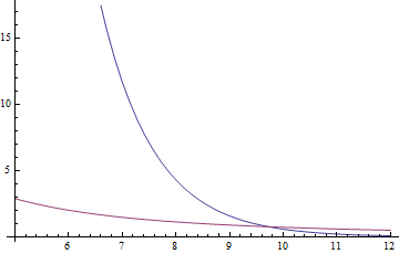
enter image description here

restoring the original definitions we get:
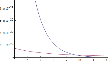
enter image description here

this result is machine precision

9.724519615727882`

the result I get rationalizing everything (ie. rationalizing each input quantity and never doing any floating operations ) and using FindRoot[ WorkingPrecision->100 ] is

9.72451961572788227332283528658...

you would be hard pressed to explain how the high precision result is somehow meaningful.

Here is a case where you should take a close look at the magniture of your quantities and do some manipulation to normalize things before throwing the system at the computer:

  Zl = 2.05*10^-15
  α = 1.6381
  ρ = 0.326*10^-10
  k = 8.9875517873681764*10^9
  e = 1.602176565*10^\[Minus]19

divide both of your expressions by ( ρ e ) :

  f1[x_] = Zl  Exp[-x] / e 
  f2[x_] = α k e/x^2/ρ 

note by the way there is no need for delayed definitions here. note also I did this by hand, you do not want an expression with e^2 / e

the expression you are solving is now fairly tame: f1[x]==f2[x]

12795.1 E^-x == 72.356/x^2

 NSolve[ f1[x] == f2[x], x]

{{x -> -0.0725216}, {x -> 0.0781981}, {x -> 9.72452}}

with a warning that there could be other solutions, but you can easily convince yourself that there are not.

 Plot[{ f1[x] , f2[x] } , {x, 5, 12}]

enter image description here

restoring the original definitions we get:

enter image description here

this result is machine precision

9.724519615727882`

the result I get rationalizing everything (ie. rationalizing each input quantity and never doing any floating operations ) and using FindRoot[ WorkingPrecision->100 ] is

9.72451961572788227332283528658...

you would be hard pressed to explain how the high precision result is somehow meaningful.

Here is a case where you should take a close look at the magnitude of your quantities and do some manipulation to normalize things before throwing the system at the computer:

  Zl = 2.05*10^-15
  α = 1.6381
  ρ = 0.326*10^-10
  k = 8.9875517873681764*10^9
  e = 1.602176565*10^\[Minus]19

divide both of your expressions by ( ρ e ) :

  f1[x_] = Zl  Exp[-x] / e 
  f2[x_] = α k e/x^2/ρ 

note by the way there is no need for delayed definitions here. note also I did this by hand, you do not want an expression with e^2 / e

the expression you are solving is now fairly tame: f1[x]==f2[x]

12795.1 E^-x == 72.356/x^2

 NSolve[ f1[x] == f2[x], x]

{{x -> -0.0725216}, {x -> 0.0781981}, {x -> 9.72452}}

with a warning that there could be other solutions, but you can easily convince yourself that there are not.

 Plot[{ f1[x] , f2[x] } , {x, 5, 12}]

enter image description here

restoring the original definitions we get:

enter image description here

this result is machine precision

9.724519615727882`

the result I get rationalizing everything (ie. rationalizing each input quantity and never doing any floating operations ) and using FindRoot[ WorkingPrecision->100 ] is

9.72451961572788227332283528658...

you would be hard pressed to explain how the high precision result is somehow meaningful.

Here is a case where you should take a close look at the magniture of your quantities and do some manipulation to normalize things before throwing the system at the computer:

  Zl = 2.05*10^-15
  \[Alpha]α = 1.6381
  \[Rho]ρ = 0.326*10^-10
  k = 8.9875517873681764*10^9
  e = 1.602176565*10^\[Minus]19

divide both of your expressions by ( \[Rho]ρ e ) :

  f1[x_] = Zl  Exp[-x] / e 
  f2[x_] = \[Alpha]α k e/x^2/\[Rho]ρ 

note by the way there is no need for delayed definitions here. note also I did this by hand, you do not want an expression with e^2 / e

the expression you are solving is now fairly tame: f1[x]==f2[x]

12795.1 E^-x == 72.356/x^2

 NSolve[ f1[x] == f2[x], x]

{{x -> -0.0725216}, {x -> 0.0781981}, {x -> 9.72452}}

with a warning that there could be other solutions, but you can easily convince yourself that there are not.

 Plot[{ f1[x] , f2[x] } , {x, 5, 12}]

enter image description here

restoring the original definitions we get:

enter image description here

this result is machine precision

9.724519615727882`

the result I get rationalizing everything (ie. rationalizing each input quantity and never doing any floating operations ) and using FindRoot[ WorkingPrecision->100 ] is

9.72451961572788227332283528658...

you would be hard pressed to explain how the high precision result is somehow meaningful.

Here is a case where you should take a close look at the magniture of your quantities and do some manipulation to normalize things before throwing the system at the computer:

  Zl = 2.05*10^-15
  \[Alpha] = 1.6381
  \[Rho] = 0.326*10^-10
  k = 8.9875517873681764*10^9
  e = 1.602176565*10^\[Minus]19

divide both of your expressions by ( \[Rho] e ) :

  f1[x_] = Zl  Exp[-x] / e 
  f2[x_] = \[Alpha] k e/x^2/\[Rho] 

note by the way there is no need for delayed definitions here. note also I did this by hand, you do not want an expression with e^2 / e

the expression you are solving is now fairly tame: f1[x]==f2[x]

12795.1 E^-x == 72.356/x^2

 NSolve[ f1[x] == f2[x], x]

{{x -> -0.0725216}, {x -> 0.0781981}, {x -> 9.72452}}

with a warning that there could be other solutions, but you can easily convince yourself that there are not.

 Plot[{ f1[x] , f2[x] } , {x, 5, 12}]

enter image description here

restoring the original definitions we get:

enter image description here

this result is machine precision

9.724519615727882`

the result I get rationalizing everything (ie. rationalizing each input quantity and never doing any floating operations ) and using FindRoot[ WorkingPrecision->100 ] is

9.72451961572788227332283528658...

you would be hard pressed to explain how the high precision result is somehow meaningful.

Here is a case where you should take a close look at the magniture of your quantities and do some manipulation to normalize things before throwing the system at the computer:

  Zl = 2.05*10^-15
  α = 1.6381
  ρ = 0.326*10^-10
  k = 8.9875517873681764*10^9
  e = 1.602176565*10^\[Minus]19

divide both of your expressions by ( ρ e ) :

  f1[x_] = Zl  Exp[-x] / e 
  f2[x_] = α k e/x^2/ρ 

note by the way there is no need for delayed definitions here. note also I did this by hand, you do not want an expression with e^2 / e

the expression you are solving is now fairly tame: f1[x]==f2[x]

12795.1 E^-x == 72.356/x^2

 NSolve[ f1[x] == f2[x], x]

{{x -> -0.0725216}, {x -> 0.0781981}, {x -> 9.72452}}

with a warning that there could be other solutions, but you can easily convince yourself that there are not.

 Plot[{ f1[x] , f2[x] } , {x, 5, 12}]

enter image description here

restoring the original definitions we get:

enter image description here

this result is machine precision

9.724519615727882`

the result I get rationalizing everything (ie. rationalizing each input quantity and never doing any floating operations ) and using FindRoot[ WorkingPrecision->100 ] is

9.72451961572788227332283528658...

you would be hard pressed to explain how the high precision result is somehow meaningful.

Source Link
george2079
  • 39.1k
  • 1
  • 44
  • 111

Here is a case where you should take a close look at the magniture of your quantities and do some manipulation to normalize things before throwing the system at the computer:

  Zl = 2.05*10^-15
  \[Alpha] = 1.6381
  \[Rho] = 0.326*10^-10
  k = 8.9875517873681764*10^9
  e = 1.602176565*10^\[Minus]19

divide both of your expressions by ( \[Rho] e ) :

  f1[x_] = Zl  Exp[-x] / e 
  f2[x_] = \[Alpha] k e/x^2/\[Rho] 

note by the way there is no need for delayed definitions here. note also I did this by hand, you do not want an expression with e^2 / e

the expression you are solving is now fairly tame: f1[x]==f2[x]

12795.1 E^-x == 72.356/x^2

 NSolve[ f1[x] == f2[x], x]

{{x -> -0.0725216}, {x -> 0.0781981}, {x -> 9.72452}}

with a warning that there could be other solutions, but you can easily convince yourself that there are not.

 Plot[{ f1[x] , f2[x] } , {x, 5, 12}]

enter image description here

restoring the original definitions we get:

enter image description here

this result is machine precision

9.724519615727882`

the result I get rationalizing everything (ie. rationalizing each input quantity and never doing any floating operations ) and using FindRoot[ WorkingPrecision->100 ] is

9.72451961572788227332283528658...

you would be hard pressed to explain how the high precision result is somehow meaningful.