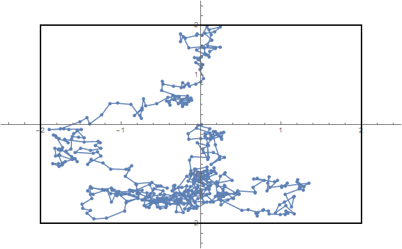
I chose the WienerProcess as the underlying random process, as this will simulate a Brownian motion.
Until Boundary Hit
Module[{rd = Transpose @ RandomFunction[WienerProcess[], {0, 1000, .01}, 2]["States"], length},
length = LengthWhile[rd, # \[Element]∈ Rectangle[{-2, -2}, {+2, +2}] &];
ListPlot[rd[[;; length]], Joined -> True, Mesh -> All, PlotRange -> {{-2.5, 2.5}, {-2.5, 2.5}},
Epilog -> {EdgeForm[Thick], White, Opacity[0], Rectangle[{-2, -2}, {+2, +2}]}, ImageSize -> Large]
]

Other Direction Inside the Boundary
First the single moves as definded by a WienerProcess:
randomMove = Transpose[Differences /@
               RandomFunction[WienerProcess[], {0, 100, .1}, 2]["States"]];
These are
Length@randomMove
1000
steps.
We'll start at
start = {0., 0.};
and define the boundary as a square
box2D = Rectangle[{-2, -2}, {+2, +2}];
Now the random walk is inside this box is created with:
last = start;
walk = First@Last@Reap@Do[
new = last + randomMove[[i]];
If[new \[Element]∈ box2D,
last = new;
Sow@new, Null],
{i, Length@randomMove}
];
randomInTheBox = Prepend[walk, start];
In my last run these where
Length@randomInTheBox
882
points.
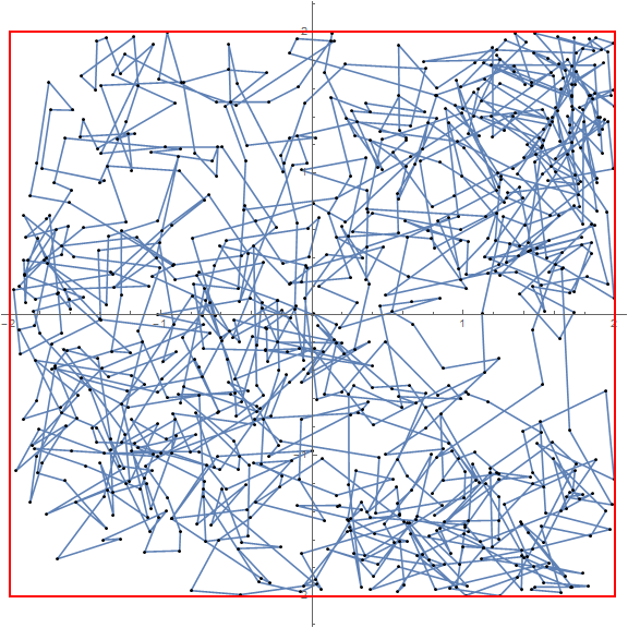
A plot of the result:
ListPlot[randomInTheBox, Joined -> True, Mesh -> All, MeshStyle -> Black, AspectRatio -> 1,
  Epilog -> {EdgeForm[{Thick, Red}], White, Opacity[0],
             Rectangle[{-2, -2}, {+2, +2}]}, ImageSize -> Large]

The walk can be traced with
Manipulate[ListPlot[randomInTheBox, Joined -> True, Mesh -> All,
  MeshStyle -> Black, AspectRatio -> 1,
  Epilog -> {PointSize[Medium], Red, Point[randomInTheBox[[p]]],
             EdgeForm[{Thick, Red}], Opacity[0], box2D}],
 {p, 1, Length@randomInTheBox, 1}]
The random process can easily replaced by an other one and a different definition for the bounding area be chosen. Furthermore an extension of this approach to 3D is straight forward.


