typo
Source Link
ciao
  • 26k
  • 2
  • 61
  • 142

It is almost always a bad idea to generate random variates one at a time in a time-sensitive construct in MM. This is a rudimentary way of doing a sim. run, with a million variates queued up:

len = 15
box = 2^len - 1
cnt = 1
Catch[Scan[(If[(box = BitXor[box, #]) == 0, Throw[cnt], cnt++]) &, 
   2^RandomInteger[len - 1, 1000000]]] 

Folding it instead of scanning may well be faster.

If you want to solve directly, say for the case of a box of six:

d = DiscreteMarkovProcess[1, {
    {0, 1, 0, 0, 0, 0, 0},
    {1/6, 0, 5/6, 0, 0, 0, 0},
    {0, 2/6, 0, 4/6, 0, 0, 0},
    {0, 0, 3/6, 0, 3/6, 0, 0},
    {0, 0, 0, 4/6, 0, 2/6, 0},
    {0, 0, 0, 0, 5/6, 0, 1/6},
    {0, 0, 0, 0, 0, 0, 1}
   }];

Mean[FirstPassageTimeDistribution[d, 7]]

(* 416/5 *)

For the general solution:

size[n_] := Module[{mp, sa},
   sa = SparseArray[{Band[{2, 1}] -> Range[1/n, (n - 1)/n, 1/n], 
      Band[{2, 3}] -> Range[(n - 1)/n, 1/n, -1/n], {1, 2} -> 
       1, {n + 1, n + 1} -> 1}, {n + 1, n + 1}];
   mp = DiscreteMarkovProcess[1, sa];
   {mp,Mean[FirstPassageTimeDistribution[mp, n + 1]]}];

s=size[20]

(* 3234139734016/2909907 *)

Which takes only a fraction of a second even on the netbook I'm on right now.

With the returned process, you can do all kinds of sorcery, like graph how many bits wherewere 1 on the way to all 1's:

d = s[[1]];
f = RandomFunction[d, {1, 5000}];
ListLinePlot[f]
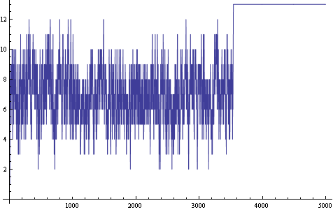
enter image description here

It is almost always a bad idea to generate random variates one at a time in a time-sensitive construct in MM. This is a rudimentary way of doing a sim. run, with a million variates queued up:

len = 15
box = 2^len - 1
cnt = 1
Catch[Scan[(If[(box = BitXor[box, #]) == 0, Throw[cnt], cnt++]) &, 
   2^RandomInteger[len - 1, 1000000]]] 

Folding it instead of scanning may well be faster.

If you want to solve directly, say for the case of a box of six:

d = DiscreteMarkovProcess[1, {
    {0, 1, 0, 0, 0, 0, 0},
    {1/6, 0, 5/6, 0, 0, 0, 0},
    {0, 2/6, 0, 4/6, 0, 0, 0},
    {0, 0, 3/6, 0, 3/6, 0, 0},
    {0, 0, 0, 4/6, 0, 2/6, 0},
    {0, 0, 0, 0, 5/6, 0, 1/6},
    {0, 0, 0, 0, 0, 0, 1}
   }];

Mean[FirstPassageTimeDistribution[d, 7]]

(* 416/5 *)

For the general solution:

size[n_] := Module[{mp, sa},
   sa = SparseArray[{Band[{2, 1}] -> Range[1/n, (n - 1)/n, 1/n], 
      Band[{2, 3}] -> Range[(n - 1)/n, 1/n, -1/n], {1, 2} -> 
       1, {n + 1, n + 1} -> 1}, {n + 1, n + 1}];
   mp = DiscreteMarkovProcess[1, sa];
   {mp,Mean[FirstPassageTimeDistribution[mp, n + 1]]}];

s=size[20]

(* 3234139734016/2909907 *)

Which takes only a fraction of a second even on the netbook I'm on right now.

With the returned process, you can do all kinds of sorcery, like graph how many bits where 1 on the way to all 1's:

d = s[[1]];
f = RandomFunction[d, {1, 5000}];
ListLinePlot[f]

enter image description here

It is almost always a bad idea to generate random variates one at a time in a time-sensitive construct in MM. This is a rudimentary way of doing a sim. run, with a million variates queued up:

len = 15
box = 2^len - 1
cnt = 1
Catch[Scan[(If[(box = BitXor[box, #]) == 0, Throw[cnt], cnt++]) &, 
   2^RandomInteger[len - 1, 1000000]]] 

Folding it instead of scanning may well be faster.

If you want to solve directly, say for the case of a box of six:

d = DiscreteMarkovProcess[1, {
    {0, 1, 0, 0, 0, 0, 0},
    {1/6, 0, 5/6, 0, 0, 0, 0},
    {0, 2/6, 0, 4/6, 0, 0, 0},
    {0, 0, 3/6, 0, 3/6, 0, 0},
    {0, 0, 0, 4/6, 0, 2/6, 0},
    {0, 0, 0, 0, 5/6, 0, 1/6},
    {0, 0, 0, 0, 0, 0, 1}
   }];

Mean[FirstPassageTimeDistribution[d, 7]]

(* 416/5 *)

For the general solution:

size[n_] := Module[{mp, sa},
   sa = SparseArray[{Band[{2, 1}] -> Range[1/n, (n - 1)/n, 1/n], 
      Band[{2, 3}] -> Range[(n - 1)/n, 1/n, -1/n], {1, 2} -> 
       1, {n + 1, n + 1} -> 1}, {n + 1, n + 1}];
   mp = DiscreteMarkovProcess[1, sa];
   {mp,Mean[FirstPassageTimeDistribution[mp, n + 1]]}];

s=size[20]

(* 3234139734016/2909907 *)

Which takes only a fraction of a second even on the netbook I'm on right now.

With the returned process, you can do all kinds of sorcery, like graph how many bits were 1 on the way to all 1's:

d = s[[1]];
f = RandomFunction[d, {1, 5000}];
ListLinePlot[f]

enter image description here

Added process graphics
Source Link
ciao
  • 26k
  • 2
  • 61
  • 142

It is almost always a bad idea to generate random variates one at a time in a time-sensitive construct in MM. This is a rudimentary way of doing a sim. run, with a million variates queued up:

len = 15
box = 2^len - 1
cnt = 1
Catch[Scan[(If[(box = BitXor[box, #]) == 0, Throw[cnt], cnt++]) &, 
   2^RandomInteger[len - 1, 1000000]]] 

Folding it instead of scanning may well be faster.

If you want to solve directly, say for the case of a box of six:

d = DiscreteMarkovProcess[1, {
    {0, 1, 0, 0, 0, 0, 0},
    {1/6, 0, 5/6, 0, 0, 0, 0},
    {0, 2/6, 0, 4/6, 0, 0, 0},
    {0, 0, 3/6, 0, 3/6, 0, 0},
    {0, 0, 0, 4/6, 0, 2/6, 0},
    {0, 0, 0, 0, 5/6, 0, 1/6},
    {0, 0, 0, 0, 0, 0, 1}
   }];

Mean[FirstPassageTimeDistribution[d, 7]]

(* 416/5 *)

For the general solution:

size[n_] := Module[{mp, sa},
   sa = SparseArray[{Band[{2, 1}] -> Range[1/n, (n - 1)/n, 1/n], 
      Band[{2, 3}] -> Range[(n - 1)/n, 1/n, -1/n], {1, 2} -> 
       1, {n + 1, n + 1} -> 1}, {n + 1, n + 1}];
   mp = DiscreteMarkovProcess[1, sa];
   {mp,Mean[FirstPassageTimeDistribution[mp, n + 1]]];1]]}];

size[20]s=size[20]

(* 3234139734016/2909907 *)

Which takes only a fraction of a second even on the netbook I'm on right now.

With the returned process, you can do all kinds of sorcery, like graph how many bits where 1 on the way to all 1's:

d = s[[1]];
f = RandomFunction[d, {1, 5000}];
ListLinePlot[f]

enter image description here

It is almost always a bad idea to generate random variates one at a time in a time-sensitive construct in MM. This is a rudimentary way of doing a sim. run, with a million variates queued up:

len = 15
box = 2^len - 1
cnt = 1
Catch[Scan[(If[(box = BitXor[box, #]) == 0, Throw[cnt], cnt++]) &, 
   2^RandomInteger[len - 1, 1000000]]] 

Folding it instead of scanning may well be faster.

If you want to solve directly, say for the case of a box of six:

d = DiscreteMarkovProcess[1, {
    {0, 1, 0, 0, 0, 0, 0},
    {1/6, 0, 5/6, 0, 0, 0, 0},
    {0, 2/6, 0, 4/6, 0, 0, 0},
    {0, 0, 3/6, 0, 3/6, 0, 0},
    {0, 0, 0, 4/6, 0, 2/6, 0},
    {0, 0, 0, 0, 5/6, 0, 1/6},
    {0, 0, 0, 0, 0, 0, 1}
   }];

Mean[FirstPassageTimeDistribution[d, 7]]

(* 416/5 *)

For the general solution:

size[n_] := Module[{mp, sa},
   sa = SparseArray[{Band[{2, 1}] -> Range[1/n, (n - 1)/n, 1/n], 
      Band[{2, 3}] -> Range[(n - 1)/n, 1/n, -1/n], {1, 2} -> 
       1, {n + 1, n + 1} -> 1}, {n + 1, n + 1}];
   mp = DiscreteMarkovProcess[1, sa];
   Mean[FirstPassageTimeDistribution[mp, n + 1]]];

size[20]

(* 3234139734016/2909907 *)

Which takes only a fraction of a second even on the netbook I'm on right now.

It is almost always a bad idea to generate random variates one at a time in a time-sensitive construct in MM. This is a rudimentary way of doing a sim. run, with a million variates queued up:

len = 15
box = 2^len - 1
cnt = 1
Catch[Scan[(If[(box = BitXor[box, #]) == 0, Throw[cnt], cnt++]) &, 
   2^RandomInteger[len - 1, 1000000]]] 

Folding it instead of scanning may well be faster.

If you want to solve directly, say for the case of a box of six:

d = DiscreteMarkovProcess[1, {
    {0, 1, 0, 0, 0, 0, 0},
    {1/6, 0, 5/6, 0, 0, 0, 0},
    {0, 2/6, 0, 4/6, 0, 0, 0},
    {0, 0, 3/6, 0, 3/6, 0, 0},
    {0, 0, 0, 4/6, 0, 2/6, 0},
    {0, 0, 0, 0, 5/6, 0, 1/6},
    {0, 0, 0, 0, 0, 0, 1}
   }];

Mean[FirstPassageTimeDistribution[d, 7]]

(* 416/5 *)

For the general solution:

size[n_] := Module[{mp, sa},
   sa = SparseArray[{Band[{2, 1}] -> Range[1/n, (n - 1)/n, 1/n], 
      Band[{2, 3}] -> Range[(n - 1)/n, 1/n, -1/n], {1, 2} -> 
       1, {n + 1, n + 1} -> 1}, {n + 1, n + 1}];
   mp = DiscreteMarkovProcess[1, sa];
   {mp,Mean[FirstPassageTimeDistribution[mp, n + 1]]}];

s=size[20]

(* 3234139734016/2909907 *)

Which takes only a fraction of a second even on the netbook I'm on right now.

With the returned process, you can do all kinds of sorcery, like graph how many bits where 1 on the way to all 1's:

d = s[[1]];
f = RandomFunction[d, {1, 5000}];
ListLinePlot[f]

enter image description here

Added general method
Source Link
ciao
  • 26k
  • 2
  • 61
  • 142

It is almost always a bad idea to generate random variates one at a time in a time-sensitive construct in MM. This is a rudimentary way of doing a sim. run, with a million variates queued up:

len = 15
box = 2^len - 1
cnt = 1
Catch[Scan[(If[(box = BitXor[box, #]) == 0, Throw[cnt], cnt++]) &, 
   2^RandomInteger[len - 1, 1000000]]] 

Folding it instead of scanning may well be faster.

If you want to solve directly, say for the case of a box of six:

d = DiscreteMarkovProcess[1, {
    {0, 1, 0, 0, 0, 0, 0},
    {1/6, 0, 5/6, 0, 0, 0, 0},
    {0, 2/6, 0, 4/6, 0, 0, 0},
    {0, 0, 3/6, 0, 3/6, 0, 0},
    {0, 0, 0, 4/6, 0, 2/6, 0},
    {0, 0, 0, 0, 5/6, 0, 1/6},
    {0, 0, 0, 0, 0, 0, 1}
   }];

Mean[FirstPassageTimeDistribution[d, 7]]

(* 416/5 *)

For the general solution:

size[n_] := Module[{mp, sa},
   sa = SparseArray[{Band[{2, 1}] -> Range[1/n, (n - 1)/n, 1/n], 
      Band[{2, 3}] -> Range[(n - 1)/n, 1/n, -1/n], {1, 2} -> 
       1, {n + 1, n + 1} -> 1}, {n + 1, n + 1}];
   mp = DiscreteMarkovProcess[1, sa];
   Mean[FirstPassageTimeDistribution[mp, n + 1]]];

size[20]

(* 3234139734016/2909907 *)

Which takes only a fraction of a second even on the netbook I'm on right now.

It is almost always a bad idea to generate random variates one at a time in a time-sensitive construct in MM. This is a rudimentary way of doing a sim. run, with a million variates queued up:

len = 15
box = 2^len - 1
cnt = 1
Catch[Scan[(If[(box = BitXor[box, #]) == 0, Throw[cnt], cnt++]) &, 
   2^RandomInteger[len - 1, 1000000]]] 

Folding it instead of scanning may well be faster.

If you want to solve directly, say for the case of a box of six:

d = DiscreteMarkovProcess[1, {
    {0, 1, 0, 0, 0, 0, 0},
    {1/6, 0, 5/6, 0, 0, 0, 0},
    {0, 2/6, 0, 4/6, 0, 0, 0},
    {0, 0, 3/6, 0, 3/6, 0, 0},
    {0, 0, 0, 4/6, 0, 2/6, 0},
    {0, 0, 0, 0, 5/6, 0, 1/6},
    {0, 0, 0, 0, 0, 0, 1}
   }];

Mean[FirstPassageTimeDistribution[d, 7]]

(* 416/5 *)

For the general solution:

size[n_] := Module[{mp, sa},
   sa = SparseArray[{Band[{2, 1}] -> Range[1/n, (n - 1)/n, 1/n], 
      Band[{2, 3}] -> Range[(n - 1)/n, 1/n, -1/n], {1, 2} -> 
       1, {n + 1, n + 1} -> 1}, {n + 1, n + 1}];
   mp = DiscreteMarkovProcess[1, sa];
   Mean[FirstPassageTimeDistribution[mp, n + 1]]];

size[20]

(* 3234139734016/2909907 *)

Which takes only a fraction of a second even on the netbook I'm on right now.

Added solution method.
Source Link
ciao
  • 26k
  • 2
  • 61
  • 142
Loading
Source Link
ciao
  • 26k
  • 2
  • 61
  • 142
Loading