Corrected the indexing of snd to get sndData.
Source Link
Anjan Kumar
  • 5k
  • 1
  • 17
  • 29

Get a sample sound:

snd = ExampleData[{"Sound", "SopranoSaxophone"}];

This gives us a Sound data structure with a SampledSoundList as first element. Extracting the data from it:

sndData = snd[[1, 1, 1]];
sndSampleRate = snd[[1, 2]];

Plotting the data:

ListPlot[sndData, DataRange -> {0, Length[sndData]/sndSampleRate }, 
 ImageSize -> 600, Frame -> True, 
 FrameLabel -> {"Time (s)", "Amplitude", "", ""}, 
 BaseStyle -> {FontFamily -> "Arial", FontWeight -> Bold, 14}]
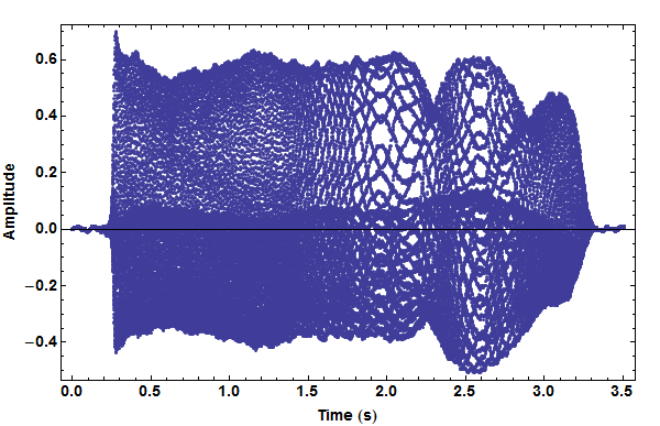
Mathematica graphics

Find the lowest amplitude level (used as reference for dB calculations):

min = Min[Abs[Fourier[sndData]]];

A spectrogram is made by making a DFT of partitions of the sample. The partitions usually have some overlap.

partSize = 2500;
offset = 250;
spectroGramData = 
  Take[20*Log10[Abs[Fourier[#]]/min], {2, partSize/2 // Floor}] & /@ 
   Partition[sndData, partSize, offset];

Note that I skip the first element of the DFT. This is the mean level. I also show only half of the frequency data. Because of the finite sampling only half of the returned coefficient list contains useful frequency information (up to the Nyquist frequency).

MatrixPlot[
  Reverse[spectroGramData\[Transpose]], 
  ColorFunction -> "Rainbow", 
  DataRange -> 
    Round[
     {{0, Length[sndData]/sndSampleRate }, 
     {sndSampleRate/partSize, sndSampleRate/2 }}, 
     0.1
    ], 
  AspectRatio -> 1/2,  ImageSize -> 800, 
  Frame -> True, FrameLabel -> {"Frequency (Hz)", "Time (s)", "", ""}, 
  BaseStyle -> {FontFamily -> "Arial", FontWeight -> Bold, 12}
]
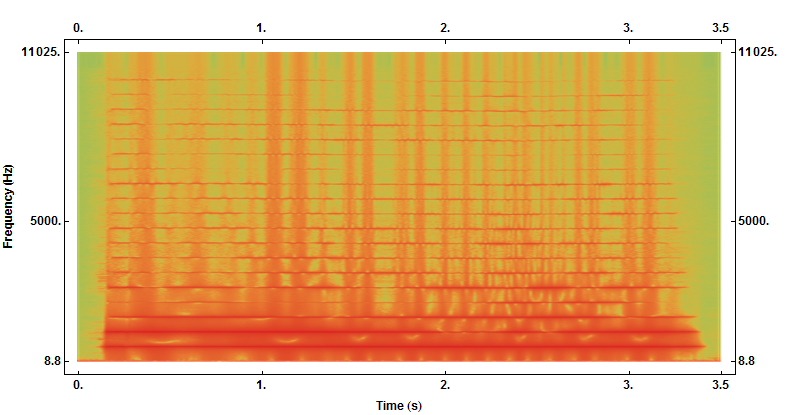
Mathematica graphics

A 3D spectrogram (note the different offset value):

partSize = 2500;
offset = 2500;
spectroGramData = 
  Take[20*Log10[Abs[Fourier[#]]/min], {2, partSize/2 // Floor}] & /@ 
   Partition[sndData, partSize, offset];

ListPlot3D[spectroGramData\[Transpose], ColorFunction -> "Rainbow", 
 DataRange -> 
  Round[{{0, Length[sndData]/sndSampleRate }, {sndSampleRate/partSize,
      sndSampleRate/2}}, 0.1], ImageSize -> 800, 
 BaseStyle -> {FontFamily -> "Arial", FontWeight -> Bold, 12}]
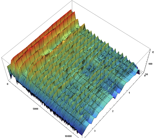
Mathematica graphics

Get a sample sound:

snd = ExampleData[{"Sound", "SopranoSaxophone"}];

This gives us a Sound data structure with a SampledSoundList as first element. Extracting the data from it:

sndData = snd[[1, 1, 1]];
sndSampleRate = snd[[1, 2]];

Plotting the data:

ListPlot[sndData, DataRange -> {0, Length[sndData]/sndSampleRate }, 
 ImageSize -> 600, Frame -> True, 
 FrameLabel -> {"Time (s)", "Amplitude", "", ""}, 
 BaseStyle -> {FontFamily -> "Arial", FontWeight -> Bold, 14}]

Mathematica graphics

Find the lowest amplitude level (used as reference for dB calculations):

min = Min[Abs[Fourier[sndData]]];

A spectrogram is made by making a DFT of partitions of the sample. The partitions usually have some overlap.

partSize = 2500;
offset = 250;
spectroGramData = 
  Take[20*Log10[Abs[Fourier[#]]/min], {2, partSize/2 // Floor}] & /@ 
   Partition[sndData, partSize, offset];

Note that I skip the first element of the DFT. This is the mean level. I also show only half of the frequency data. Because of the finite sampling only half of the returned coefficient list contains useful frequency information (up to the Nyquist frequency).

MatrixPlot[
  Reverse[spectroGramData\[Transpose]], 
  ColorFunction -> "Rainbow", 
  DataRange -> 
    Round[
     {{0, Length[sndData]/sndSampleRate }, 
     {sndSampleRate/partSize, sndSampleRate/2 }}, 
     0.1
    ], 
  AspectRatio -> 1/2,  ImageSize -> 800, 
  Frame -> True, FrameLabel -> {"Frequency (Hz)", "Time (s)", "", ""}, 
  BaseStyle -> {FontFamily -> "Arial", FontWeight -> Bold, 12}
]

Mathematica graphics

A 3D spectrogram (note the different offset value):

partSize = 2500;
offset = 2500;
spectroGramData = 
  Take[20*Log10[Abs[Fourier[#]]/min], {2, partSize/2 // Floor}] & /@ 
   Partition[sndData, partSize, offset];

ListPlot3D[spectroGramData\[Transpose], ColorFunction -> "Rainbow", 
 DataRange -> 
  Round[{{0, Length[sndData]/sndSampleRate }, {sndSampleRate/partSize,
      sndSampleRate/2}}, 0.1], ImageSize -> 800, 
 BaseStyle -> {FontFamily -> "Arial", FontWeight -> Bold, 12}]

Mathematica graphics

Get a sample sound:

snd = ExampleData[{"Sound", "SopranoSaxophone"}];

This gives us a Sound data structure with a SampledSoundList as first element. Extracting the data from it:

sndData = snd[[1, 1]];
sndSampleRate = snd[[1, 2]];

Plotting the data:

ListPlot[sndData, DataRange -> {0, Length[sndData]/sndSampleRate }, 
 ImageSize -> 600, Frame -> True, 
 FrameLabel -> {"Time (s)", "Amplitude", "", ""}, 
 BaseStyle -> {FontFamily -> "Arial", FontWeight -> Bold, 14}]

Mathematica graphics

Find the lowest amplitude level (used as reference for dB calculations):

min = Min[Abs[Fourier[sndData]]];

A spectrogram is made by making a DFT of partitions of the sample. The partitions usually have some overlap.

partSize = 2500;
offset = 250;
spectroGramData = 
  Take[20*Log10[Abs[Fourier[#]]/min], {2, partSize/2 // Floor}] & /@ 
   Partition[sndData, partSize, offset];

Note that I skip the first element of the DFT. This is the mean level. I also show only half of the frequency data. Because of the finite sampling only half of the returned coefficient list contains useful frequency information (up to the Nyquist frequency).

MatrixPlot[
  Reverse[spectroGramData\[Transpose]], 
  ColorFunction -> "Rainbow", 
  DataRange -> 
    Round[
     {{0, Length[sndData]/sndSampleRate }, 
     {sndSampleRate/partSize, sndSampleRate/2 }}, 
     0.1
    ], 
  AspectRatio -> 1/2,  ImageSize -> 800, 
  Frame -> True, FrameLabel -> {"Frequency (Hz)", "Time (s)", "", ""}, 
  BaseStyle -> {FontFamily -> "Arial", FontWeight -> Bold, 12}
]

Mathematica graphics

A 3D spectrogram (note the different offset value):

partSize = 2500;
offset = 2500;
spectroGramData = 
  Take[20*Log10[Abs[Fourier[#]]/min], {2, partSize/2 // Floor}] & /@ 
   Partition[sndData, partSize, offset];

ListPlot3D[spectroGramData\[Transpose], ColorFunction -> "Rainbow", 
 DataRange -> 
  Round[{{0, Length[sndData]/sndSampleRate }, {sndSampleRate/partSize,
      sndSampleRate/2}}, 0.1], ImageSize -> 800, 
 BaseStyle -> {FontFamily -> "Arial", FontWeight -> Bold, 12}]

Mathematica graphics

added missing }
Source Link
Sjoerd C. de Vries
  • 66.1k
  • 15
  • 189
  • 327

Get a sample sound:

snd = ExampleData[{"Sound", "SopranoSaxophone"}];

This gives us a Sound data structure with a SampledSoundList as first element. Extracting the data from it:

sndData = snd[[1, 1, 1]];
sndSampleRate = snd[[1, 2]];

Plotting the data:

ListPlot[sndData, DataRange -> {0, Length[sndData]/sndSampleRate }, 
 ImageSize -> 600, Frame -> True, 
 FrameLabel -> {"Time (s)", "Amplitude", "", ""}, 
 BaseStyle -> {FontFamily -> "Arial", FontWeight -> Bold, 14}]

Mathematica graphics

Find the lowest amplitude level (used as reference for dB calculations):

min = Min[Abs[Fourier[sndData]]];

A spectrogram is made by making a DFT of partitions of the sample. The partitions usually have some overlap.

partSize = 2500;
offset = 250;
spectroGramData = 
  Take[20*Log10[Abs[Fourier[#]]/min], {2, partSize/2 // Floor}] & /@ 
   Partition[sndData, partSize, offset];

Note that I skip the first element of the DFT. This is the mean level. I also show only half of the frequency data. Because of the finite sampling only half of the returned coefficient list contains useful frequency information (up to the Nyquist frequency).

MatrixPlot[
  Reverse[spectroGramData\[Transpose]], 
  ColorFunction -> "Rainbow", 
  DataRange -> 
    Round[
     {{0, Length[sndData]/sndSampleRate }, 
     {sndSampleRate/partSize, sndSampleRate/2 }}, 
     0.1
    ], 
  AspectRatio -> 1/2,  ImageSize -> 800, 
  Frame -> True, FrameLabel -> {"Frequency (Hz)", "Time (s)", "", ""}, 
  BaseStyle -> {FontFamily -> "Arial", FontWeight -> Bold, 12}
]

Mathematica graphics

A 3D spectrogram (note the different offset value):

partSize = 2500;
offset = 2500;
spectroGramData = 
  Take[20*Log10[Abs[Fourier[#]]/min], {2, partSize/2 // Floor}] & /@ 
   Partition[sndData, partSize, offset];

ListPlot3D[spectroGramData\[Transpose], ColorFunction -> "Rainbow", 
 DataRange -> 
  Round[{{0, Length[sndData]/sndSampleRate }, {sndSampleRate/partSize,
      sndSampleRate/2}}, 0.1], ImageSize -> 800, 
 BaseStyle -> {FontFamily -> "Arial", FontWeight -> Bold, 12}]

Mathematica graphics

Get a sample sound:

snd = ExampleData[{"Sound", "SopranoSaxophone"}];

This gives us a Sound data structure with a SampledSoundList as first element. Extracting the data from it:

sndData = snd[[1, 1, 1]];
sndSampleRate = snd[[1, 2]];

Plotting the data:

ListPlot[sndData, DataRange -> {0, Length[sndData]/sndSampleRate }, 
 ImageSize -> 600, Frame -> True, 
 FrameLabel -> {"Time (s)", "Amplitude", "", ""}, 
 BaseStyle -> {FontFamily -> "Arial", FontWeight -> Bold, 14}]

Mathematica graphics

Find the lowest amplitude level (used as reference for dB calculations):

min = Min[Abs[Fourier[sndData]]];

A spectrogram is made by making a DFT of partitions of the sample. The partitions usually have some overlap.

partSize = 2500;
offset = 250;
spectroGramData = 
  Take[20*Log10[Abs[Fourier[#]]/min], {2, partSize/2 // Floor}] & /@ 
   Partition[sndData, partSize, offset];

Note that I skip the first element of the DFT. This is the mean level. I also show only half of the frequency data. Because of the finite sampling only half of the returned coefficient list contains useful frequency information (up to the Nyquist frequency).

MatrixPlot[
  Reverse[spectroGramData\[Transpose]], 
  ColorFunction -> "Rainbow", 
  DataRange -> 
    Round[
     {{0, Length[sndData]/sndSampleRate }, 
     {sndSampleRate/partSize, sndSampleRate/2 }}, 
     0.1
    ], 
  AspectRatio -> 1/2,  ImageSize -> 800, 
  Frame -> True, FrameLabel -> {"Frequency (Hz)", "Time (s)", "", ""}, 
  BaseStyle -> {FontFamily -> "Arial", FontWeight -> Bold, 12
]

Mathematica graphics

A 3D spectrogram (note the different offset value):

partSize = 2500;
offset = 2500;
spectroGramData = 
  Take[20*Log10[Abs[Fourier[#]]/min], {2, partSize/2 // Floor}] & /@ 
   Partition[sndData, partSize, offset];

ListPlot3D[spectroGramData\[Transpose], ColorFunction -> "Rainbow", 
 DataRange -> 
  Round[{{0, Length[sndData]/sndSampleRate }, {sndSampleRate/partSize,
      sndSampleRate/2}}, 0.1], ImageSize -> 800, 
 BaseStyle -> {FontFamily -> "Arial", FontWeight -> Bold, 12}]

Mathematica graphics

Get a sample sound:

snd = ExampleData[{"Sound", "SopranoSaxophone"}];

This gives us a Sound data structure with a SampledSoundList as first element. Extracting the data from it:

sndData = snd[[1, 1, 1]];
sndSampleRate = snd[[1, 2]];

Plotting the data:

ListPlot[sndData, DataRange -> {0, Length[sndData]/sndSampleRate }, 
 ImageSize -> 600, Frame -> True, 
 FrameLabel -> {"Time (s)", "Amplitude", "", ""}, 
 BaseStyle -> {FontFamily -> "Arial", FontWeight -> Bold, 14}]

Mathematica graphics

Find the lowest amplitude level (used as reference for dB calculations):

min = Min[Abs[Fourier[sndData]]];

A spectrogram is made by making a DFT of partitions of the sample. The partitions usually have some overlap.

partSize = 2500;
offset = 250;
spectroGramData = 
  Take[20*Log10[Abs[Fourier[#]]/min], {2, partSize/2 // Floor}] & /@ 
   Partition[sndData, partSize, offset];

Note that I skip the first element of the DFT. This is the mean level. I also show only half of the frequency data. Because of the finite sampling only half of the returned coefficient list contains useful frequency information (up to the Nyquist frequency).

MatrixPlot[
  Reverse[spectroGramData\[Transpose]], 
  ColorFunction -> "Rainbow", 
  DataRange -> 
    Round[
     {{0, Length[sndData]/sndSampleRate }, 
     {sndSampleRate/partSize, sndSampleRate/2 }}, 
     0.1
    ], 
  AspectRatio -> 1/2,  ImageSize -> 800, 
  Frame -> True, FrameLabel -> {"Frequency (Hz)", "Time (s)", "", ""}, 
  BaseStyle -> {FontFamily -> "Arial", FontWeight -> Bold, 12}
]

Mathematica graphics

A 3D spectrogram (note the different offset value):

partSize = 2500;
offset = 2500;
spectroGramData = 
  Take[20*Log10[Abs[Fourier[#]]/min], {2, partSize/2 // Floor}] & /@ 
   Partition[sndData, partSize, offset];

ListPlot3D[spectroGramData\[Transpose], ColorFunction -> "Rainbow", 
 DataRange -> 
  Round[{{0, Length[sndData]/sndSampleRate }, {sndSampleRate/partSize,
      sndSampleRate/2}}, 0.1], ImageSize -> 800, 
 BaseStyle -> {FontFamily -> "Arial", FontWeight -> Bold, 12}]

Mathematica graphics

added 189 characters in body
Source Link
Sjoerd C. de Vries
  • 66.1k
  • 15
  • 189
  • 327

Get a sample sound:

snd = ExampleData[{"Sound", "SopranoSaxophone"}];

This gives us a Sound data structure with a SampledSoundList as first element. Extracting the data from it:

sndData = snd[[1, 1, 1]];
sndSampleRate = snd[[1, 2]];

Plotting the data:

ListPlot[sndData, DataRange -> {0, Length[sndData]/sndSampleRate }, 
 ImageSize -> 600, Frame -> True, 
 FrameLabel -> {"Time (s)", "Amplitude", "", ""}, 
 BaseStyle -> {FontFamily -> "Arial", FontWeight -> Bold, 14}]

Mathematica graphics

Find the lowest amplitude level (used as reference for dB calculations):

min = Min[Abs[Fourier[sndData]]];

A spectrogram is made by making a DFT of partitions of the sample. The partitions usually have some overlap.

partSize = 2500;
offset = 250;
spectroGramData = 
  Take[20*Log10[Abs[Fourier[#]]/min], {2, partSize/2 // Floor}] & /@ 
   Partition[sndData, partSize, offset];

Note that I skip the first element of the DFT. This is the mean level. I also show only half of the frequency data. Because of the finite sampling only half of the returned coefficient list contains useful frequency information (up to the Nyquist frequency).

MatrixPlot[
  Reverse[spectroGramData\[Transpose]], 
  ColorFunction -> "Rainbow", 
  DataRange -> 
    Round[
     {{0, Length[sndData]/sndSampleRate }, 
     {sndSampleRate/partSize, sndSampleRate/2 }}, 
     0.1
    ], 
  AspectRatio -> 1/2,  ImageSize -> 800, 
  Frame -> True, FrameLabel -> {"Frequency (Hz)", "Time (s)", "", ""}, 
  BaseStyle -> {FontFamily -> "Arial", FontWeight -> Bold, 12
]

Mathematica graphics

A 3D spectrogram (note the different offset value):

partSize = 2500;
offset = 2500;
spectroGramData = 
  Take[20*Log10[Abs[Fourier[#]]/min], {2, partSize/2 // Floor}] & /@ 
   Partition[sndData, partSize, offset];

ListPlot3D[spectroGramData\[Transpose], ColorFunction -> "Rainbow", 
 DataRange -> 
  Round[{{0, Length[sndData]/sndSampleRate }, {sndSampleRate/partSize,
      sndSampleRate/2}}, 0.1], ImageSize -> 800, 
 BaseStyle -> {FontFamily -> "Arial", FontWeight -> Bold, 12}]

Mathematica graphics

Get a sample sound:

snd = ExampleData[{"Sound", "SopranoSaxophone"}];

This gives us a Sound data structure with a SampledSoundList as first element. Extracting the data from it:

sndData = snd[[1, 1, 1]];
sndSampleRate = snd[[1, 2]];

Plotting the data:

ListPlot[sndData, DataRange -> {0, Length[sndData]/sndSampleRate }, 
 ImageSize -> 600, Frame -> True, 
 FrameLabel -> {"Time (s)", "Amplitude", "", ""}, 
 BaseStyle -> {FontFamily -> "Arial", FontWeight -> Bold, 14}]

Mathematica graphics

Find the lowest amplitude level (used as reference for dB calculations):

min = Min[Abs[Fourier[sndData]]];

A spectrogram is made by making a DFT of partitions of the sample. The partitions usually have some overlap.

partSize = 2500;
offset = 250;
spectroGramData = 
  Take[20*Log10[Abs[Fourier[#]]/min], {2, partSize/2 // Floor}] & /@ 
   Partition[sndData, partSize, offset];

Note that I skip the first element of the DFT. This is the mean level. I also show only half of the frequency data. Because of the finite sampling only half of the returned coefficient list contains useful frequency information (up to the Nyquist frequency).

MatrixPlot[
  Reverse[spectroGramData\[Transpose]], 
  ColorFunction -> "Rainbow", 
  DataRange -> 
    Round[
     {{0, Length[sndData]/sndSampleRate }, 
     {sndSampleRate/partSize, sndSampleRate/2 }}, 
     0.1
    ], 
  AspectRatio -> 1/2,  ImageSize -> 800, 
  Frame -> True, FrameLabel -> {"Frequency (Hz)", "Time (s)", "", ""}, 
  BaseStyle -> {FontFamily -> "Arial", FontWeight -> Bold, 12
]

Mathematica graphics

A 3D spectrogram (note the different offset value):

partSize = 2500;
offset = 2500;
spectroGramData = 
  Take[20*Log10[Abs[Fourier[#]]/min], {2, partSize/2 // Floor}] & /@ 
   Partition[sndData, partSize, offset];

ListPlot3D[spectroGramData\[Transpose], ColorFunction -> "Rainbow", 
 DataRange -> 
  Round[{{0, Length[sndData]/sndSampleRate }, {sndSampleRate/partSize,
      sndSampleRate/2}}, 0.1], ImageSize -> 800, 
 BaseStyle -> {FontFamily -> "Arial", FontWeight -> Bold, 12}]

Mathematica graphics

added 417 characters in body
Source Link
Sjoerd C. de Vries
  • 66.1k
  • 15
  • 189
  • 327
Loading
added 1 characters in body
Source Link
Sjoerd C. de Vries
  • 66.1k
  • 15
  • 189
  • 327
Loading
Source Link
Sjoerd C. de Vries
  • 66.1k
  • 15
  • 189
  • 327
Loading