Edit - incorporating ideas from the comments

It makes sense to transform the exponential equation to both take advantage of the benefits of normalization and generate results that are on the same scale as the original data. If our model is defined by eqn below, then we can transform the equation by applying Rescale to the x and y values to get eqn2:

{xmin, xmax, ymin, ymax} = Flatten[Through[{Min, Max}[#]] & /@ Transpose@data]
eqn = y == a Exp[b x] + c
eqn2 = y /. Solve[eqn /. {y -> Rescale[y, {ymin, ymax}],
    x -> Rescale[x, {xmin, xmax}]}, y] // First
(* 1000*(45 + 166*c + 166*a*E^(b*(-182 + x/11))) *)

Performing the NonlinearModelFit with Method->NMinimize appears to be a little more forgiving with the starting values for the parameters, at the expense of a slightly longer calculation time.

nlm = NonlinearModelFit[data, eqn2, {a, b, c}, x, Method -> NMinimize]; 
Column[{
  nlm["BestFitParameters"],
  Normal[nlm],
  nlm["CorrelationMatrix"] // MatrixForm}, Left, 2]

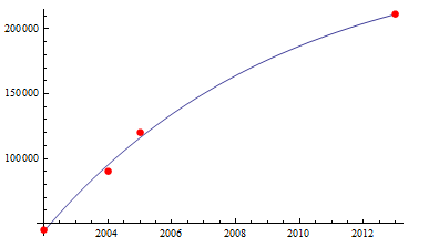
Plot[nlm[x], {x, xmin, xmax}, Epilog -> {Red, PointSize[0.02], Point /@ data}]

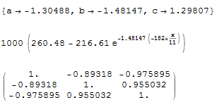
Normal provides a form of the equation that can be used to extract the values of a, b, and c, with the caveat that b is not a trivial transformation. I included the correlation matrix to point out that the parameters are highly correlated in this example, suggesting that a fit to this model may not be the best one. As an example of this point, we could also fit the data to a dosage-response function (eqn3):

eqn3 = y == a + (b - a)/(1 + (c/x));
eqn4 = y /. Solve[eqn3 /. {y -> Rescale[y, {ymin, ymax}], 
       x -> Rescale[x, {xmin, xmax}]}, y] // First;
nlm2 = NonlinearModelFit[data, eqn4, {a, b, c}, x,Method -> NMinimize];
Row[{Plot[nlm2[x], {x, xmin, xmax}, 
   Epilog -> {Red, PointSize[0.02], Point /@ data}], Column[{
    nlm2["BestFitParameters"],
    Normal[nlm2],
    nlm2["CorrelationMatrix"] // MatrixForm}, Left, 2]}]

There is less correlation between the parameters in this model, although note that b and c are fairly highly correlated. Removing c from the model (c = 1) and repeating the above process gives:

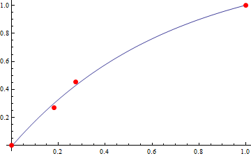
I have not looked closely at confidence intervals or goodness of fit; however a visual inspection of the three figures suggests that there is not much difference between the three models, which in my opinion leads to a conclusion that the latter model, with its small number of uncorrelated parameters, is appropriate for this set of data. Granted, this assumes no knowledge of what the data are, how they were obtained, and the theory they are supposed to follow.

Original post

I'm no stats expert, but in my experience, normalizing data that spans different orders of magnitude helps:

datan[[All, 1]] = 
 Rescale[#, {Min[data[[All, 1]]], Max[data[[All, 1]]]}] & /@ 
  data[[All, 1]]
datan[[All, 2]] = 
 Rescale[#, {Min[data[[All, 2]]], Max[data[[All, 2]]]}] & /@ 
  data[[All, 2]]
nlm = NonlinearModelFit[datan, a Exp[b x] + c, {a, b, c}, x]
Plot[nlm[x], {x, 0, 1}, 
 Epilog -> {Red, PointSize[0.02], Point /@ datan}, PlotRange -> All]

I'm no stats expert, but in my experience, normalizing data that spans different orders of magnitude helps:

datan[[All, 1]] = Rescale[#, {Min[data[[All, 1]]], Max[data[[All, 1]]]}] & /@  data[[All, 1]]
datan[[All, 2]] = Rescale[#, {Min[data[[All, 2]]], Max[data[[All, 2]]]}] & /@  data[[All, 2]]
nlm = NonlinearModelFit[datan, a Exp[b x] + c, {a, b, c}, x]
Plot[nlm[x], {x, 0, 1}, Epilog -> {Red, PointSize[0.02], Point /@ datan}, PlotRange -> All]