added 201 characters in body
Source Link
Bob Hanlon
  • 162.7k
  • 7
  • 81
  • 205
$Version

(* "14.0.0 for Mac OS X ARM (64-bit) (December 13, 2023)" *)

Clear["Global`*"]

f = (E^(-(s/lm))  v  (lm - 
       2  lm  Hypergeometric2F1[1, -(lg/lm), 1 - lg/lm, E^(s/lg)] - 
       2  E^(s/lm)  (s - lg  Log[1 - E^(s/lg)])))/H /. {H -> 0.1, v -> 0.5, 
   lg -> 1, lm -> 2}

(* 5. E^(-s/2) (2 - 4 Hypergeometric2F1[-(1/2), 1, 1/2, E^s] - 
   2 E^(s/2) (s - Log[1 - E^s])) *)

If you are getting imaginary artifacts with your version, try using exact values and simplifying.

f2 = (E^(-(s/lm))  v  (lm - 
         2  lm  Hypergeometric2F1[1, -(lg/lm), 1 - lg/lm, E^(s/lg)] - 
         2  E^(s/lm)  (s - lg  Log[1 - E^(s/lg)])))/H /. {H -> 1/10, v -> 1/2,
      lg -> 1, lm -> 2} // FunctionExpand // Simplify

(* 10 (-E^(-s/2) - s + 2 E^(-s/2) Sqrt[E^s] ArcTanh[Sqrt[E^s]] + Log[1 - E^s]) *)

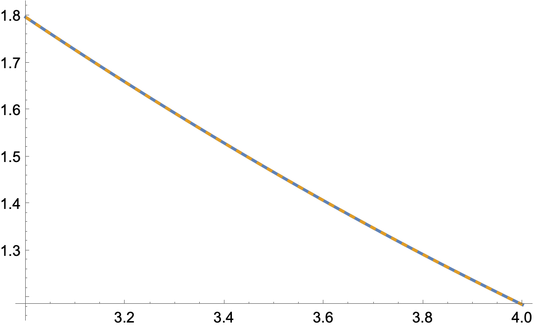
Both plots are continuous

Plot[{f, f2}, {s, 3, 4},
 PlotStyle -> {Automatic, Dashed}]

enter image description here

EDIT: Or for a more robust solution, use ComplexExpand with f2

f3 = Assuming[s > 0, 
  f2 // ComplexExpand[#, TargetFunctions -> {Re, Im}] & // Simplify]

(* 10 (-E^(-s/2) - s + 2 Log[1 + E^(s/2)]) *)

FunctionDomain[f3, s]

(* True *)

Although f3 was developed assuming s > 0, f3 == f2 for real s

Assuming[s ∈ Reals, 
 ComplexExpand[f2 == f3, TargetFunctions -> {Re, Im}] // FullSimplify]

(* True *)
$Version

(* "14.0.0 for Mac OS X ARM (64-bit) (December 13, 2023)" *)

Clear["Global`*"]

f = (E^(-(s/lm))  v  (lm - 
       2  lm  Hypergeometric2F1[1, -(lg/lm), 1 - lg/lm, E^(s/lg)] - 
       2  E^(s/lm)  (s - lg  Log[1 - E^(s/lg)])))/H /. {H -> 0.1, v -> 0.5, 
   lg -> 1, lm -> 2}

(* 5. E^(-s/2) (2 - 4 Hypergeometric2F1[-(1/2), 1, 1/2, E^s] - 
   2 E^(s/2) (s - Log[1 - E^s])) *)

If you are getting imaginary artifacts with your version, try using exact values and simplifying.

f2 = (E^(-(s/lm))  v  (lm - 
         2  lm  Hypergeometric2F1[1, -(lg/lm), 1 - lg/lm, E^(s/lg)] - 
         2  E^(s/lm)  (s - lg  Log[1 - E^(s/lg)])))/H /. {H -> 1/10, v -> 1/2,
      lg -> 1, lm -> 2} // FunctionExpand // Simplify

(* 10 (-E^(-s/2) - s + 2 E^(-s/2) Sqrt[E^s] ArcTanh[Sqrt[E^s]] + Log[1 - E^s]) *)

Both plots are continuous

Plot[{f, f2}, {s, 3, 4},
 PlotStyle -> {Automatic, Dashed}]

enter image description here

EDIT: Or for a more robust solution, use ComplexExpand with f2

f3 = Assuming[s > 0, 
  f2 // ComplexExpand[#, TargetFunctions -> {Re, Im}] & // Simplify]

(* 10 (-E^(-s/2) - s + 2 Log[1 + E^(s/2)]) *)

FunctionDomain[f3, s]

(* True *)

Although f3 was developed assuming s > 0, f3 == f2 for real s

Assuming[s ∈ Reals, 
 ComplexExpand[f2 == f3, TargetFunctions -> {Re, Im}] // FullSimplify]

(* True *)
Added use of ComplexExpand
Source Link
Bob Hanlon
  • 162.7k
  • 7
  • 81
  • 205
$Version

(* "14.0.0 for Mac OS X ARM (64-bit) (December 13, 2023)" *)

Clear["Global`*"]

f = (E^(-(s/lm))  v  (lm - 
       2  lm  Hypergeometric2F1[1, -(lg/lm), 1 - lg/lm, E^(s/lg)] - 
       2  E^(s/lm)  (s - lg  Log[1 - E^(s/lg)])))/H /. {H -> 0.1, v -> 0.5, 
   lg -> 1, lm -> 2}

(* 5. E^(-s/2) (2 - 4 Hypergeometric2F1[-(1/2), 1, 1/2, E^s] - 
   2 E^(s/2) (s - Log[1 - E^s])) *)

If you are getting imaginary artifacts with your version, try using exact values and simplifying.

f2 = (E^(-(s/lm))  v  (lm - 
         2  lm  Hypergeometric2F1[1, -(lg/lm), 1 - lg/lm, E^(s/lg)] - 
         2  E^(s/lm)  (s - lg  Log[1 - E^(s/lg)])))/H /. {H -> 1/10, v -> 1/2,
      lg -> 1, lm -> 2} // FunctionExpand // Simplify

(* 10 (-E^(-s/2) - s + 2 E^(-s/2) Sqrt[E^s] ArcTanh[Sqrt[E^s]] + Log[1 - E^s]) *)

Both plots are continuous

Plot[{f, f2}, {s, 3, 4},
 PlotStyle -> {Automatic, Dashed}]

enter image description here

EDIT: Or for a more robust solution, use ComplexExpand with f2

f3 = Assuming[s > 0, 
  f2 // ComplexExpand[#, TargetFunctions -> {Re, Im}] & // Simplify]

(* 10 (-E^(-s/2) - s + 2 Log[1 + E^(s/2)]) *)

FunctionDomain[f3, s]

(* True *)
$Version

(* "14.0.0 for Mac OS X ARM (64-bit) (December 13, 2023)" *)

Clear["Global`*"]

f = (E^(-(s/lm))  v  (lm - 
       2  lm  Hypergeometric2F1[1, -(lg/lm), 1 - lg/lm, E^(s/lg)] - 
       2  E^(s/lm)  (s - lg  Log[1 - E^(s/lg)])))/H /. {H -> 0.1, v -> 0.5, 
   lg -> 1, lm -> 2}

(* 5. E^(-s/2) (2 - 4 Hypergeometric2F1[-(1/2), 1, 1/2, E^s] - 
   2 E^(s/2) (s - Log[1 - E^s])) *)

If you are getting imaginary artifacts with your version, try using exact values and simplifying.

f2 = (E^(-(s/lm))  v  (lm - 
         2  lm  Hypergeometric2F1[1, -(lg/lm), 1 - lg/lm, E^(s/lg)] - 
         2  E^(s/lm)  (s - lg  Log[1 - E^(s/lg)])))/H /. {H -> 1/10, v -> 1/2,
      lg -> 1, lm -> 2} // FunctionExpand // Simplify

(* 10 (-E^(-s/2) - s + 2 E^(-s/2) Sqrt[E^s] ArcTanh[Sqrt[E^s]] + Log[1 - E^s]) *)

Both plots are continuous

Plot[{f, f2}, {s, 3, 4},
 PlotStyle -> {Automatic, Dashed}]

enter image description here

EDIT: Or for a more robust solution, use ComplexExpand with f2

f3 = Assuming[s > 0, 
  f2 // ComplexExpand[#, TargetFunctions -> {Re, Im}] & // Simplify]

(* 10 (-E^(-s/2) - s + 2 Log[1 + E^(s/2)]) *)

FunctionDomain[f3, s]

(* True *)
Source Link
Bob Hanlon
  • 162.7k
  • 7
  • 81
  • 205

$Version

(* "14.0.0 for Mac OS X ARM (64-bit) (December 13, 2023)" *)

Clear["Global`*"]

f = (E^(-(s/lm))  v  (lm - 
       2  lm  Hypergeometric2F1[1, -(lg/lm), 1 - lg/lm, E^(s/lg)] - 
       2  E^(s/lm)  (s - lg  Log[1 - E^(s/lg)])))/H /. {H -> 0.1, v -> 0.5, 
   lg -> 1, lm -> 2}

(* 5. E^(-s/2) (2 - 4 Hypergeometric2F1[-(1/2), 1, 1/2, E^s] - 
   2 E^(s/2) (s - Log[1 - E^s])) *)

If you are getting imaginary artifacts with your version, try using exact values and simplifying.

f2 = (E^(-(s/lm))  v  (lm - 
         2  lm  Hypergeometric2F1[1, -(lg/lm), 1 - lg/lm, E^(s/lg)] - 
         2  E^(s/lm)  (s - lg  Log[1 - E^(s/lg)])))/H /. {H -> 1/10, v -> 1/2,
      lg -> 1, lm -> 2} // FunctionExpand // Simplify

(* 10 (-E^(-s/2) - s + 2 E^(-s/2) Sqrt[E^s] ArcTanh[Sqrt[E^s]] + Log[1 - E^s]) *)

Both plots are continuous

Plot[{f, f2}, {s, 3, 4},
 PlotStyle -> {Automatic, Dashed}]

enter image description here