Revisions to How to construct a contour plot so that positive contour lines are colored red and negative contour lines are colored blue

added 203 characters in body

Source Link

edited Apr 20 at 16:45

25.1k
2
22
62

Update:

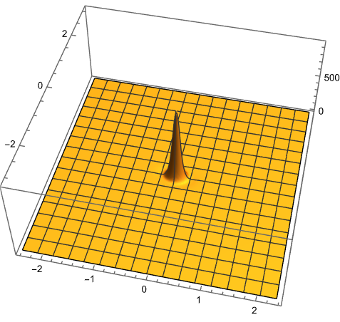
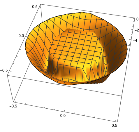
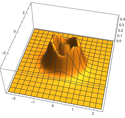
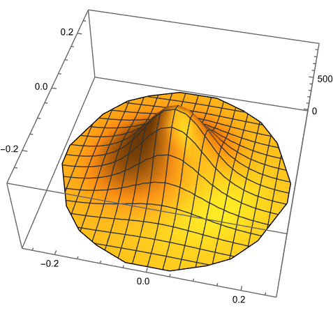
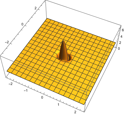
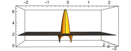
Here is a depiction of the data by ListPlot3D. The data can be separated into three groups by the third value.

On the first image the whole data is used but all that can be seen is just the positive data with #[[3]] > 0.46 because the other values are to small compared to it.

On the next three images you can see data from the three groups separately.

data = Import["planeImageData[Import["https://i.txt"sstatic.net/TMXaHoiJ.png"], "Table"][[All,"Byte"] {1,// 2, 
 4}]];  Flatten // FromCharacterCode // Uncompress;
ListPlot3D[data, PlotRange -> All]
ListPlot3D[Select[data, #[[3]] < 0 &], PlotRange -> All]
ListPlot3D[Select[data, 0 < #[[3]] < 0.46 &], PlotRange -> All]
ListPlot3D[Select[data, #[[3]] > 0.46 &], PlotRange -> All]

Another way to depict the data is to use logarithm on third value so that details of each group of data are visible.

ListPlot3D[{#[[1]], #[[2]], Log[#[[3]] + 6]} & /@ data, 
 PlotRange -> All]

Original answer:

data = Flatten[
   Table[{x, y, x^2 - (y)^2}, {x, -1, 1, 0.1}, {y, -1, 1, 0.1}], 1];
mm = MinMax@data[[All, 3]];
d = 0.1;
cont = Table[{Rescale[k, {0, 1}, mm], 
    Blend[{Blue, White, Red}, k]}, {k, 0, 1, d/(mm[[2]] - mm[[1]])}];
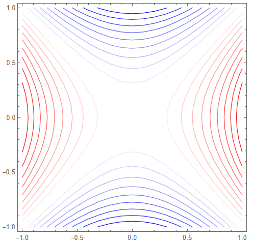
ListContourPlot[data, ContourShading -> None, Contours -> cont]

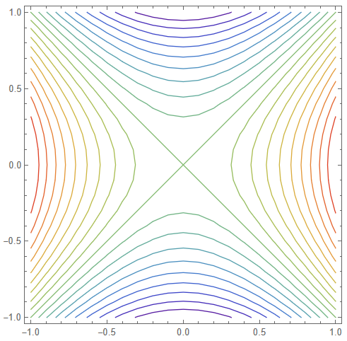
With ColorData["Rainbow"][k] instead of Blend[{Blue, White, Red}, k].

With If[k < 0.5, Blue, Red] instead of Blend[{Blue, White, Red}, k].

data stored in image:

Update:

Here is a depiction of the data by ListPlot3D. The data can be separated into three groups by the third value.

On the first image the whole data is used but all that can be seen is just the positive data with #[[3]] > 0.46 because the other values are to small compared to it.

On the next three images you can see data from the three groups separately.

data = Import["plane.txt", "Table"][[All, {1, 2, 4}]];
ListPlot3D[data, PlotRange -> All]
ListPlot3D[Select[data, #[[3]] < 0 &], PlotRange -> All]
ListPlot3D[Select[data, 0 < #[[3]] < 0.46 &], PlotRange -> All]
ListPlot3D[Select[data, #[[3]] > 0.46 &], PlotRange -> All]

Another way to depict the data is to use logarithm on third value so that details of each group of data are visible.

ListPlot3D[{#[[1]], #[[2]], Log[#[[3]] + 6]} & /@ data, 
 PlotRange -> All]

Original answer:

data = Flatten[
   Table[{x, y, x^2 - (y)^2}, {x, -1, 1, 0.1}, {y, -1, 1, 0.1}], 1];
mm = MinMax@data[[All, 3]];
d = 0.1;
cont = Table[{Rescale[k, {0, 1}, mm], 
    Blend[{Blue, White, Red}, k]}, {k, 0, 1, d/(mm[[2]] - mm[[1]])}];
ListContourPlot[data, ContourShading -> None, Contours -> cont]

With ColorData["Rainbow"][k] instead of Blend[{Blue, White, Red}, k].

With If[k < 0.5, Blue, Red] instead of Blend[{Blue, White, Red}, k].

Update:

Here is a depiction of the data by ListPlot3D. The data can be separated into three groups by the third value.

On the first image the whole data is used but all that can be seen is just the positive data with #[[3]] > 0.46 because the other values are to small compared to it.

On the next three images you can see data from the three groups separately.

data = ImageData[Import["https://i.sstatic.net/TMXaHoiJ.png"], "Byte"] //  
   Flatten // FromCharacterCode // Uncompress;
ListPlot3D[data, PlotRange -> All]
ListPlot3D[Select[data, #[[3]] < 0 &], PlotRange -> All]
ListPlot3D[Select[data, 0 < #[[3]] < 0.46 &], PlotRange -> All]
ListPlot3D[Select[data, #[[3]] > 0.46 &], PlotRange -> All]

Another way to depict the data is to use logarithm on third value so that details of each group of data are visible.

ListPlot3D[{#[[1]], #[[2]], Log[#[[3]] + 6]} & /@ data, 
 PlotRange -> All]

Original answer:

data = Flatten[
   Table[{x, y, x^2 - (y)^2}, {x, -1, 1, 0.1}, {y, -1, 1, 0.1}], 1];
mm = MinMax@data[[All, 3]];
d = 0.1;
cont = Table[{Rescale[k, {0, 1}, mm], 
    Blend[{Blue, White, Red}, k]}, {k, 0, 1, d/(mm[[2]] - mm[[1]])}];
ListContourPlot[data, ContourShading -> None, Contours -> cont]

With ColorData["Rainbow"][k] instead of Blend[{Blue, White, Red}, k].

With If[k < 0.5, Blue, Red] instead of Blend[{Blue, White, Red}, k].

data stored in image:

added 1441 characters in body

Source Link

edited Apr 20 at 16:07

azerbajdzan

25.1k
2
22
62

Update:

Here is a depiction of the data by ListPlot3D. The data can be separated into three groups by the third value.

On the first image the whole data is used but all that can be seen is just the positive data with #[[3]] > 0.46 because the other values are to small compared to it.

On the next three images you can see data from the three groups separately.

data = Import["plane.txt", "Table"][[All, {1, 2, 4}]];
ListPlot3D[data, PlotRange -> All]
ListPlot3D[Select[data, #[[3]] < 0 &], PlotRange -> All]
ListPlot3D[Select[data, 0 < #[[3]] < 0.46 &], PlotRange -> All]
ListPlot3D[Select[data, #[[3]] > 0.46 &], PlotRange -> All]

Another way to depict the data is to use logarithm on third value so that details of each group of data are visible.

ListPlot3D[{#[[1]], #[[2]], Log[#[[3]] + 6]} & /@ data, 
 PlotRange -> All]

Original answer:

data = Flatten[
   Table[{x, y, x^2 - (y)^2}, {x, -1, 1, 0.1}, {y, -1, 1, 0.1}], 1];
mm = MinMax@data[[All, 3]];
d = 0.1;
cont = Table[{Rescale[k, {0, 1}, mm], 
    Blend[{Blue, White, Red}, k]}, {k, 0, 1, d/(mm[[2]] - mm[[1]])}];
ListContourPlot[data, ContourShading -> None, Contours -> cont]

With ColorData["Rainbow"][k] instead of Blend[{Blue, White, Red}, k].

With If[k < 0.5, Blue, Red] instead of Blend[{Blue, White, Red}, k].

data = Flatten[
   Table[{x, y, x^2 - (y)^2}, {x, -1, 1, 0.1}, {y, -1, 1, 0.1}], 1];
mm = MinMax@data[[All, 3]];
d = 0.1;
cont = Table[{Rescale[k, {0, 1}, mm], 
    Blend[{Blue, White, Red}, k]}, {k, 0, 1, d/(mm[[2]] - mm[[1]])}];
ListContourPlot[data, ContourShading -> None, Contours -> cont]

With ColorData["Rainbow"][k] instead of Blend[{Blue, White, Red}, k].

With If[k < 0.5, Blue, Red] instead of Blend[{Blue, White, Red}, k].

Update:

Here is a depiction of the data by ListPlot3D. The data can be separated into three groups by the third value.

On the first image the whole data is used but all that can be seen is just the positive data with #[[3]] > 0.46 because the other values are to small compared to it.

On the next three images you can see data from the three groups separately.

data = Import["plane.txt", "Table"][[All, {1, 2, 4}]];
ListPlot3D[data, PlotRange -> All]
ListPlot3D[Select[data, #[[3]] < 0 &], PlotRange -> All]
ListPlot3D[Select[data, 0 < #[[3]] < 0.46 &], PlotRange -> All]
ListPlot3D[Select[data, #[[3]] > 0.46 &], PlotRange -> All]

Another way to depict the data is to use logarithm on third value so that details of each group of data are visible.

ListPlot3D[{#[[1]], #[[2]], Log[#[[3]] + 6]} & /@ data, 
 PlotRange -> All]

Original answer:

data = Flatten[
   Table[{x, y, x^2 - (y)^2}, {x, -1, 1, 0.1}, {y, -1, 1, 0.1}], 1];
mm = MinMax@data[[All, 3]];
d = 0.1;
cont = Table[{Rescale[k, {0, 1}, mm], 
    Blend[{Blue, White, Red}, k]}, {k, 0, 1, d/(mm[[2]] - mm[[1]])}];
ListContourPlot[data, ContourShading -> None, Contours -> cont]

With ColorData["Rainbow"][k] instead of Blend[{Blue, White, Red}, k].

With If[k < 0.5, Blue, Red] instead of Blend[{Blue, White, Red}, k].

deleted 48 characters in body

Source Link

edited Apr 18 at 19:58

azerbajdzan

25.1k
2
22
62

Two versions:

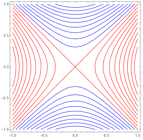
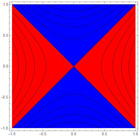
negative values are blue, positive values are red

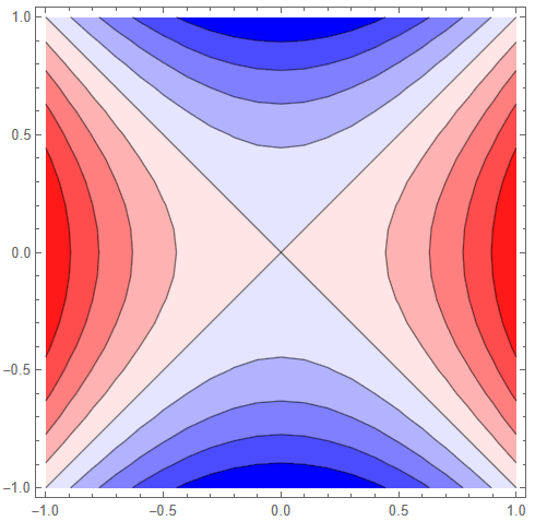
the more negative the more blueish, the more positive the more reddish

data = Flatten[
   Table[{x, y, x^2 - y^2(y)^2}, {x, -1, 1, 0.1}, {y, -1, 1, 0.1}], 1];
 
ListContourPlot[data,mm ColorFunction= ->MinMax@data[[All, (If[#3]];
d >= 0, Red,.1;
cont Blue]= &)Table[{Rescale[k, 
 ColorFunctionScaling{0, ->1}, False]

ListContourPlot[datamm], 
 ColorFunction -> ( Blend[{Blue, White, Red}, #]k]}, &{k, 0, 1, d/(mm[[2]] - mm[[1]])]}];
ListContourPlot[data, ContourShading -> None, Contours -> cont]

With ColorData["Rainbow"][k] instead of Blend[{Blue, White, Red}, k].

With If[k < 0.5, Blue, Red] instead of Blend[{Blue, White, Red}, k].

Two versions:

negative values are blue, positive values are red

the more negative the more blueish, the more positive the more reddish

data = Flatten[
   Table[{x, y, x^2 - y^2}, {x, -1, 1, 0.1}, {y, -1, 1, 0.1}], 1];
 
ListContourPlot[data, ColorFunction -> (If[# > 0, Red, Blue] &), 
 ColorFunctionScaling -> False]

ListContourPlot[data, 
 ColorFunction -> (Blend[{Blue, White, Red}, #] &)]

data = Flatten[
   Table[{x, y, x^2 - (y)^2}, {x, -1, 1, 0.1}, {y, -1, 1, 0.1}], 1];
mm = MinMax@data[[All, 3]];
d = 0.1;
cont = Table[{Rescale[k, {0, 1}, mm], 
    Blend[{Blue, White, Red}, k]}, {k, 0, 1, d/(mm[[2]] - mm[[1]])}];
ListContourPlot[data, ContourShading -> None, Contours -> cont]

With ColorData["Rainbow"][k] instead of Blend[{Blue, White, Red}, k].

With If[k < 0.5, Blue, Red] instead of Blend[{Blue, White, Red}, k].

Source Link

created Apr 18 at 18:38

azerbajdzan

25.1k
2
22
62

Loading

Stack Exchange Network

Return to Answer