added 429 characters in body
Source Link
ydd
  • 6.9k
  • 1
  • 9
  • 25

I couldn't get your code to run to generate your function, so let's just use a standard normal distribution pdf as our example function to find FWHM with.

f[x_] = PDF[NormalDistribution[], x];

We'll start by maximizing the function, and getting the value at the max along with the coordinate of the maximum:

{maxVal, maxPos} = FindMaximum[f[x], x];
maxPos = maxPos // Values // First;

And then get the positions where the function reaches half its max on both the left and right sides of the peak, and taking the difference between the two to get the FWHM:

left = NArgMin[{(f[x] - 0.5 maxVal)^2, x <= maxPos}, x];
right = NArgMin[{(f[x] - 0.5 maxVal)^2, x >= maxPos}, x];
right - left
(*2.35482*)

Note using NArgMin might not be the most optimal way to find the half-max points. There's probably a faster way to do this

Let's put this all together as a function so we can apply it to other datasets:arbitrary functions

FWHM[f_] := (
  {maxVal, maxPos} = FindMaximum[f[x], x];
  maxPos = maxPos // Values // First;
  
  left = NArgMin[{(f[x] - 0.5 maxVal)^2, x <= maxPos}, x];
  right = NArgMin[{(f[x] - 0.5 maxVal)^2, x >= maxPos}, x];
  
  right - left
  )

Testing with noisy data

Let's try to find the FWHM of the PDF of a SmoothKernelDistribution fitted from normally distributed random data. First simulate the data and fit a SmoothKernelDistribution:

SeedRandom[1];
dat = RandomVariate[NormalDistribution[], 10^3];
ClearAll[emp]
emp[x_] = PDF[SmoothKernelDistribution[dat], x];
Plot[emp[x], {x, -3, 3}]
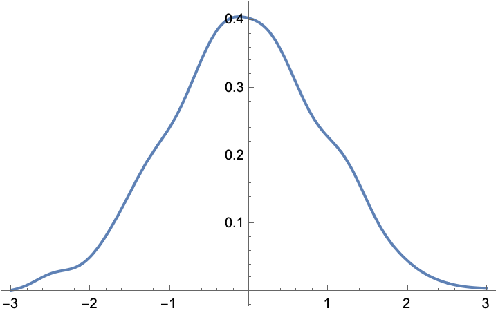
https://i.sstatic.net/1tVDO.png And now call FWHM on it. We see it's close to the theoretical FWHM value for a normal distribution $ \mathrm{FWHM} = 2 \sqrt{2 \log (2)} ~\sigma \approx 2.355 ~\sigma$ :

FWHM[emp]
(*2.41349*)

It's also worth noting: for many common "bump-like" functions, there are formula for the FWHM in terms of the function parameters, so often times you just fit the data to whatever appropriate function type, and use the fitted parameters to calculate FWHM.

I couldn't get your code to run to generate your function, so let's just use a standard normal distribution pdf as our example function to find FWHM with.

f[x_] = PDF[NormalDistribution[], x];

We'll start by maximizing the function, and getting the value at the max along with the coordinate of the maximum:

{maxVal, maxPos} = FindMaximum[f[x], x];
maxPos = maxPos // Values // First;

And then get the positions where the function reaches half its max on both the left and right sides of the peak, and taking the difference between the two to get the FWHM:

left = NArgMin[{(f[x] - 0.5 maxVal)^2, x <= maxPos}, x];
right = NArgMin[{(f[x] - 0.5 maxVal)^2, x >= maxPos}, x];
right - left
(*2.35482*)

Note using NArgMin might not be the most optimal way to find the half-max points. There's probably a faster way to do this

Let's put this all together as a function so we can apply it to other datasets:

FWHM[f_] := (
  {maxVal, maxPos} = FindMaximum[f[x], x];
  maxPos = maxPos // Values // First;
  
  left = NArgMin[{(f[x] - 0.5 maxVal)^2, x <= maxPos}, x];
  right = NArgMin[{(f[x] - 0.5 maxVal)^2, x >= maxPos}, x];
  
  right - left
  )

Testing with noisy data

Let's try to find the FWHM of the PDF of a SmoothKernelDistribution fitted from normally distributed random data. First simulate the data and fit a SmoothKernelDistribution:

SeedRandom[1];
dat = RandomVariate[NormalDistribution[], 10^3];
ClearAll[emp]
emp[x_] = PDF[SmoothKernelDistribution[dat], x];
Plot[emp[x], {x, -3, 3}]

https://i.sstatic.net/1tVDO.png And now call FWHM on it. We see it's close to the theoretical FWHM value for a normal distribution $ \mathrm{FWHM} = 2 \sqrt{2 \log (2)} ~\sigma \approx 2.355 ~\sigma$ :

FWHM[emp]
(*2.41349*)

I couldn't get your code to run to generate your function, so let's just use a standard normal distribution pdf as our example function to find FWHM with.

f[x_] = PDF[NormalDistribution[], x];

We'll start by maximizing the function, and getting the value at the max along with the coordinate of the maximum:

{maxVal, maxPos} = FindMaximum[f[x], x];
maxPos = maxPos // Values // First;

And then get the positions where the function reaches half its max on both the left and right sides of the peak, and taking the difference between the two to get the FWHM:

left = NArgMin[{(f[x] - 0.5 maxVal)^2, x <= maxPos}, x];
right = NArgMin[{(f[x] - 0.5 maxVal)^2, x >= maxPos}, x];
right - left
(*2.35482*)

Note using NArgMin might not be the most optimal way to find the half-max points. There's probably a faster way to do this

Let's put this all together as a function so we can apply it to arbitrary functions

FWHM[f_] := (
  {maxVal, maxPos} = FindMaximum[f[x], x];
  maxPos = maxPos // Values // First;
  
  left = NArgMin[{(f[x] - 0.5 maxVal)^2, x <= maxPos}, x];
  right = NArgMin[{(f[x] - 0.5 maxVal)^2, x >= maxPos}, x];
  
  right - left
  )

Testing with noisy data

Let's try to find the FWHM of the PDF of a SmoothKernelDistribution fitted from normally distributed random data. First simulate the data and fit a SmoothKernelDistribution:

SeedRandom[1];
dat = RandomVariate[NormalDistribution[], 10^3];
ClearAll[emp]
emp[x_] = PDF[SmoothKernelDistribution[dat], x];
Plot[emp[x], {x, -3, 3}]

https://i.sstatic.net/1tVDO.png And now call FWHM on it. We see it's close to the theoretical FWHM value for a normal distribution $ \mathrm{FWHM} = 2 \sqrt{2 \log (2)} ~\sigma \approx 2.355 ~\sigma$ :

FWHM[emp]
(*2.41349*)

It's also worth noting: for many common "bump-like" functions, there are formula for the FWHM in terms of the function parameters, so often times you just fit the data to whatever appropriate function type, and use the fitted parameters to calculate FWHM.

Source Link
ydd
  • 6.9k
  • 1
  • 9
  • 25

I couldn't get your code to run to generate your function, so let's just use a standard normal distribution pdf as our example function to find FWHM with.

f[x_] = PDF[NormalDistribution[], x];

We'll start by maximizing the function, and getting the value at the max along with the coordinate of the maximum:

{maxVal, maxPos} = FindMaximum[f[x], x];
maxPos = maxPos // Values // First;

And then get the positions where the function reaches half its max on both the left and right sides of the peak, and taking the difference between the two to get the FWHM:

left = NArgMin[{(f[x] - 0.5 maxVal)^2, x <= maxPos}, x];
right = NArgMin[{(f[x] - 0.5 maxVal)^2, x >= maxPos}, x];
right - left
(*2.35482*)

Note using NArgMin might not be the most optimal way to find the half-max points. There's probably a faster way to do this

Let's put this all together as a function so we can apply it to other datasets:

FWHM[f_] := (
  {maxVal, maxPos} = FindMaximum[f[x], x];
  maxPos = maxPos // Values // First;
  
  left = NArgMin[{(f[x] - 0.5 maxVal)^2, x <= maxPos}, x];
  right = NArgMin[{(f[x] - 0.5 maxVal)^2, x >= maxPos}, x];
  
  right - left
  )

Testing with noisy data

Let's try to find the FWHM of the PDF of a SmoothKernelDistribution fitted from normally distributed random data. First simulate the data and fit a SmoothKernelDistribution:

SeedRandom[1];
dat = RandomVariate[NormalDistribution[], 10^3];
ClearAll[emp]
emp[x_] = PDF[SmoothKernelDistribution[dat], x];
Plot[emp[x], {x, -3, 3}]

https://i.sstatic.net/1tVDO.png And now call FWHM on it. We see it's close to the theoretical FWHM value for a normal distribution $ \mathrm{FWHM} = 2 \sqrt{2 \log (2)} ~\sigma \approx 2.355 ~\sigma$ :

FWHM[emp]
(*2.41349*)