added 14 characters in body
Source Link
xzczd
  • 68.4k
  • 9
  • 174
  • 489

Let me add my FDM solution. The spirit of this solution is the same as that of Alex's FDM solution, except that the process is automated with pdetoode and DChange. Since there's nothing new in the following code compared to the previous moving boundary problemproblems in this site, I won't explain much. (Anyway, if you still feel it difficult to follow, feel free to ask in the comment, but please be specific. )

Let me add my FDM solution. The spirit of this solution is the same as that of Alex's FDM solution, except that the process is automated with pdetoode and DChange. Since there's nothing new in the following code compared to the previous moving boundary problem, I won't explain much. (Anyway, if you still feel it difficult to follow, feel free to ask in the comment, but please be specific. )

Let me add my FDM solution. The spirit of this solution is the same as that of Alex's FDM solution, except that the process is automated with pdetoode and DChange. Since there's nothing new in the following code compared to the previous moving boundary problems in this site, I won't explain much. (Anyway, if you still feel it difficult to follow, feel free to ask in the comment, but please be specific. )

Post Undeleted by xzczd
added 90 characters in body
Source Link
xzczd
  • 68.4k
  • 9
  • 174
  • 489

Something seems to be wrong with moving grid method. Still exploring…


Let me add amy FDM solution based on moving grid. The spirit of this solution is the same as shown in

Heat Equation with Mobile Boundary

Moving B.C.s in heat diffusion model

that of Alex's FDM solution, except that the process is automated with pdetoode and DChange. Since there's nothing new in the following code compared to the previous moving boundary problem, I won't explain much. Please read the posts linked above carefully. (Anyway, if you still feel it difficult to follow, feel free to ask in the comment, but please be specific. )

I'll use pdetoode for discretization. The initial data isI've chosen the same initial data as that chosen in Alex's answer:Alex's answer so we can easily verify the result.

s0 = 3;
F = t; v0 = x;
With[{v = v[x, t], 
   s = s[t]}, {eq, ic, 
    bc} = {{D[v, t] == D[v, x, x], 
     D[s, t] == -D[v, x] /. x -> s}, {v == v0, s == s0} /. t -> 0, {v == 0 /. x -> 0,
      D[v, x] - 1/s v == F /. x -> s}}];
(* Definition of DChange isn't included in this post,
domain   please find it in the link above. *)       
{neweq, newicmid, newbc} = DChange[{0eq, ic, bc}, x/s[t] == ξ, x, ξ, v[x, t]]    
newic = {newicmid[[1]] /. t -> 0 /. s[0] -> s0, newicmid[[2]]};

With[{ic = newic, eq = neweq, bc = newbc},
 domain = {0, 1}; points = 25;
  grid = Array[# &, points, domain];
  difforder = 2;
  (* Definition of pdetoode isn't included in this post,
     please find it in the link above. *)
  ptoofunc = pdetoode[v[xpdetoode[v[ξ, t], t, grid, difforder];
  del = #[[2 ;; -2]] &;
freeze = v[i_] 
 :> v@ToString@i(*v[i:Except[_String]]:>v@ToString@InputForm@i*);

ode = {del@ptoofunc@eq[[1]], ptoofunc@eq[[2]]};
  odebc = ptoofunc@bc;
  odeic = {ic[[1]] // ptoofunc // del, ic[[2]]} /. freeze /. t -> 0;
  tend = 1;
  {ssol, vsollst} = 
   NDSolveValue[{ode, odeic, odebc} /. freeze, {s, v /@ grid} /. freeze, {t, 0, 
     tend}]; // AbsoluteTimingAbsoluteTiming]

vscaledsol = rebuild[vsollst, grid/s[t], 2];
vsol = {x, t} |-> vscaledsol[x/ssol[t], t];
    
reg = DiscretizeRegion@ImplicitRegion[x <= ssol[t], {{t, 0, 1}, {x, 0, 3}}];

DensityPlot[vsol[x, t], {t, x} ∈ reg]

enter image description hereenter image description here

enter image description hereenter image description here

Something seems to be wrong with moving grid method. Still exploring…


Let me add a solution based on moving grid as shown in

Heat Equation with Mobile Boundary

Moving B.C.s in heat diffusion model

Since there's nothing new in the following code, I won't explain much. Please read the posts linked above carefully. (Anyway, if you still feel it difficult to follow, feel free to ask in the comment, but please be specific. )

I'll use pdetoode for discretization. The initial data is the same as that chosen in Alex's answer:

s0 = 3;
F = t; v0 = x;
With[{v = v[x, t], 
   s = s[t]}, {eq, ic, 
    bc} = {{D[v, t] == D[v, x, x], 
     D[s, t] == -D[v, x] /. x -> s}, {v == v0, s == s0} /. t -> 0, {v == 0 /. x -> 0,
      D[v, x] - 1/s v == F /. x -> s}}];

domain = {0, s[t]};
points = 25;
 grid = Array[# &, points, domain];
 difforder = 2;
(* Definition of pdetoode isn't included in this post,
   please find it in the link above. *)
ptoofunc = pdetoode[v[x, t], t, grid, difforder];
del = #[[2 ;; -2]] &;
freeze = v[i_] :> v@ToString@i(*v[i:Except[_String]]:>v@ToString@InputForm@i*);

ode = {del@ptoofunc@eq[[1]], ptoofunc@eq[[2]]};
odebc = ptoofunc@bc;
odeic = {ic[[1]] // ptoofunc // del, ic[[2]]} /. freeze /. t -> 0;
tend = 1;
{ssol, vsollst} = 
   NDSolveValue[{ode, odeic, odebc} /. freeze, {s, v /@ grid} /. freeze, {t, 0, 
     tend}]; // AbsoluteTiming

vscaledsol = rebuild[vsollst, grid/s[t], 2];
vsol = {x, t} |-> vscaledsol[x/ssol[t], t];
    
reg = DiscretizeRegion@ImplicitRegion[x <= ssol[t], {{t, 0, 1}, {x, 0, 3}}];

DensityPlot[vsol[x, t], {t, x} ∈ reg]
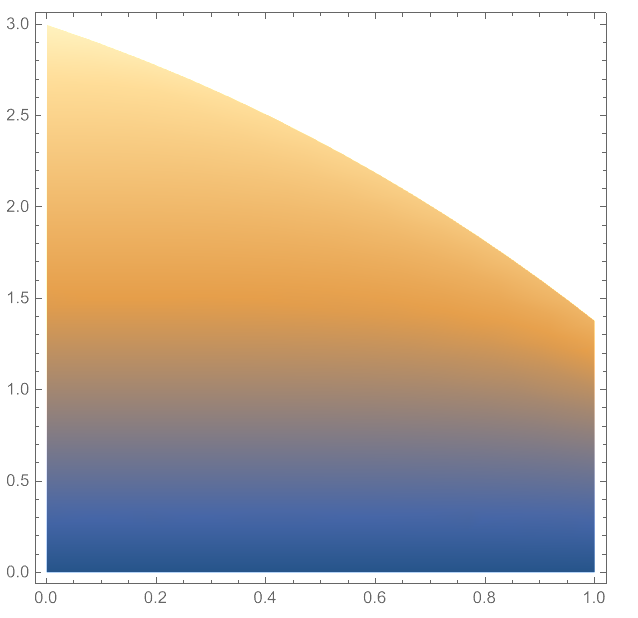
enter image description here

enter image description here

Let me add my FDM solution. The spirit of this solution is the same as that of Alex's FDM solution, except that the process is automated with pdetoode and DChange. Since there's nothing new in the following code compared to the previous moving boundary problem, I won't explain much. (Anyway, if you still feel it difficult to follow, feel free to ask in the comment, but please be specific. )

I've chosen the same initial data as in Alex's answer so we can easily verify the result.

s0 = 3;
F = t; v0 = x;
With[{v = v[x, t], 
   s = s[t]}, {eq, ic, 
    bc} = {{D[v, t] == D[v, x, x], 
     D[s, t] == -D[v, x] /. x -> s}, {v == v0, s == s0} /. t -> 0, {v == 0 /. x -> 0,
      D[v, x] - 1/s v == F /. x -> s}}];
(* Definition of DChange isn't included in this post,
   please find it in the link above. *)       
{neweq, newicmid, newbc} = DChange[{eq, ic, bc}, x/s[t] == ξ, x, ξ, v[x, t]]    
newic = {newicmid[[1]] /. t -> 0 /. s[0] -> s0, newicmid[[2]]};

With[{ic = newic, eq = neweq, bc = newbc},
 domain = {0, 1}; points = 25; grid = Array[# &, points, domain]; difforder = 2;
  (* Definition of pdetoode isn't included in this post,
     please find it in the link above. *)
  ptoofunc = pdetoode[v[ξ, t], t, grid, difforder];
  del = #[[2 ;; -2]] &;
   
  ode = {del@ptoofunc@eq[[1]], ptoofunc@eq[[2]]};
  odebc = ptoofunc@bc;
  odeic = {ic[[1]] // ptoofunc // del, ic[[2]]} /. t -> 0;
  tend = 1;
  {ssol, vsollst} = 
   NDSolveValue[{ode, odeic, odebc}, {s, v /@ grid}, {t, 0, tend}]; // AbsoluteTiming]

vscaledsol = rebuild[vsollst, grid, 2];
vsol = {x, t} |-> vscaledsol[x/ssol[t], t];
    
reg = DiscretizeRegion@ImplicitRegion[x <= ssol[t], {{t, 0, 1}, {x, 0, 3}}];

DensityPlot[vsol[x, t], {t, x} ∈ reg]

enter image description here

enter image description here

added 85 characters in body
Source Link
xzczd
  • 68.4k
  • 9
  • 174
  • 489

Something seems to be wrong with moving grid method. Still exploring…


Let me add a solution based on moving grid as shown in

Heat Equation with Mobile Boundary

Moving B.C.s in heat diffusion model

Since there's nothing new in the following code, I won't explain much. Please read the posts linked above carefully. (Anyway, if you still feel it difficult to follow, feel free to ask in the comment, but please be specific. )

I'll use pdetoode for discretization. The initial data is the same as that chosen in Alex's answer:

s0 = 3;
F = t; v0 = x;
With[{v = v[x, t], 
   s = s[t]}, {eq, ic, 
    bc} = {{D[v, t] == D[v, x, x], 
     D[s, t] == -D[v, x] /. x -> s}, {v == v0, s == s0} /. t -> 0, {v == 0 /. x -> 0,
      D[v, x] - 1/s v == F /. x -> s}}];

domain = {0, s[t]};
points = 25;
grid = Array[# &, points, domain];
difforder = 2;
(* Definition of pdetoode isn't included in this post,
   please find it in the link above. *)
ptoofunc = pdetoode[v[x, t], t, grid, difforder];
del = #[[2 ;; -2]] &;
freeze = v[i_] :> v@ToString@i(*v[i:Except[_String]]:>v@ToString@InputForm@i*);

ode = {del@ptoofunc@eq[[1]], ptoofunc@eq[[2]]};
odebc = ptoofunc@bc;
odeic = {ic[[1]] // ptoofunc // del, ic[[2]]} /. freeze /. t -> 0;
tend = 1;
{ssol, vsollst} = 
   NDSolveValue[{ode, odeic, odebc} /. freeze, {s, v /@ grid} /. freeze, {t, 0, 
     tend}]; // AbsoluteTiming

vscaledsol = rebuild[vsollst, grid/s[t], 2];
vsol = {x, t} |-> vscaledsol[x/ssol[t], t];
    
reg = DiscretizeRegion@ImplicitRegion[x <= ssol[t], {{t, 0, 1}, {x, 0, 3}}];

DensityPlot[vsol[x, t], {t, x} ∈ reg]
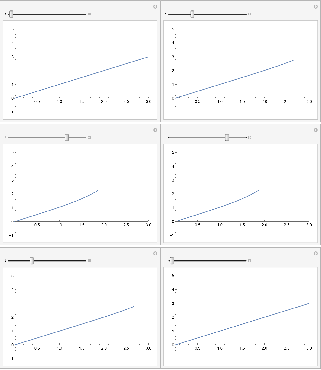
enter image description here

Manipulate[
 Plot[vsol[x, t], {x, 0, ssol[t]}, PlotRange -> {{0, s0}, {-1, 5}}], {t, 0, 1}]

enter image description here

Let me add a solution based on moving grid as shown in

Heat Equation with Mobile Boundary

Moving B.C.s in heat diffusion model

Since there's nothing new in the following code, I won't explain much. Please read the posts linked above carefully. (Anyway, if you still feel it difficult to follow, feel free to ask in the comment, but please be specific. )

I'll use pdetoode for discretization. The initial data is the same as that chosen in Alex's answer:

s0 = 3;
F = t; v0 = x;
With[{v = v[x, t], 
   s = s[t]}, {eq, ic, 
    bc} = {{D[v, t] == D[v, x, x], 
     D[s, t] == -D[v, x] /. x -> s}, {v == v0, s == s0} /. t -> 0, {v == 0 /. x -> 0,
      D[v, x] - 1/s v == F /. x -> s}}];

domain = {0, s[t]};
points = 25;
grid = Array[# &, points, domain];
difforder = 2;
(* Definition of pdetoode isn't included in this post,
   please find it in the link above. *)
ptoofunc = pdetoode[v[x, t], t, grid, difforder];
del = #[[2 ;; -2]] &;
freeze = v[i_] :> v@ToString@i(*v[i:Except[_String]]:>v@ToString@InputForm@i*);

ode = {del@ptoofunc@eq[[1]], ptoofunc@eq[[2]]};
odebc = ptoofunc@bc;
odeic = {ic[[1]] // ptoofunc // del, ic[[2]]} /. freeze /. t -> 0;
tend = 1;
{ssol, vsollst} = 
   NDSolveValue[{ode, odeic, odebc} /. freeze, {s, v /@ grid} /. freeze, {t, 0, 
     tend}]; // AbsoluteTiming

vscaledsol = rebuild[vsollst, grid/s[t], 2];
vsol = {x, t} |-> vscaledsol[x/ssol[t], t];
    
reg = DiscretizeRegion@ImplicitRegion[x <= ssol[t], {{t, 0, 1}, {x, 0, 3}}];

DensityPlot[vsol[x, t], {t, x} ∈ reg]

enter image description here

Manipulate[
 Plot[vsol[x, t], {x, 0, ssol[t]}, PlotRange -> {{0, s0}, {-1, 5}}], {t, 0, 1}]

enter image description here

Something seems to be wrong with moving grid method. Still exploring…


Let me add a solution based on moving grid as shown in

Heat Equation with Mobile Boundary

Moving B.C.s in heat diffusion model

Since there's nothing new in the following code, I won't explain much. Please read the posts linked above carefully. (Anyway, if you still feel it difficult to follow, feel free to ask in the comment, but please be specific. )

I'll use pdetoode for discretization. The initial data is the same as that chosen in Alex's answer:

s0 = 3;
F = t; v0 = x;
With[{v = v[x, t], 
   s = s[t]}, {eq, ic, 
    bc} = {{D[v, t] == D[v, x, x], 
     D[s, t] == -D[v, x] /. x -> s}, {v == v0, s == s0} /. t -> 0, {v == 0 /. x -> 0,
      D[v, x] - 1/s v == F /. x -> s}}];

domain = {0, s[t]};
points = 25;
grid = Array[# &, points, domain];
difforder = 2;
(* Definition of pdetoode isn't included in this post,
   please find it in the link above. *)
ptoofunc = pdetoode[v[x, t], t, grid, difforder];
del = #[[2 ;; -2]] &;
freeze = v[i_] :> v@ToString@i(*v[i:Except[_String]]:>v@ToString@InputForm@i*);

ode = {del@ptoofunc@eq[[1]], ptoofunc@eq[[2]]};
odebc = ptoofunc@bc;
odeic = {ic[[1]] // ptoofunc // del, ic[[2]]} /. freeze /. t -> 0;
tend = 1;
{ssol, vsollst} = 
   NDSolveValue[{ode, odeic, odebc} /. freeze, {s, v /@ grid} /. freeze, {t, 0, 
     tend}]; // AbsoluteTiming

vscaledsol = rebuild[vsollst, grid/s[t], 2];
vsol = {x, t} |-> vscaledsol[x/ssol[t], t];
    
reg = DiscretizeRegion@ImplicitRegion[x <= ssol[t], {{t, 0, 1}, {x, 0, 3}}];

DensityPlot[vsol[x, t], {t, x} ∈ reg]

enter image description here

Manipulate[
 Plot[vsol[x, t], {x, 0, ssol[t]}, PlotRange -> {{0, s0}, {-1, 5}}], {t, 0, 1}]

enter image description here

Post Deleted by xzczd
Source Link
xzczd
  • 68.4k
  • 9
  • 174
  • 489
Loading