added 273 characters in body
Source Link

If you want a symbolic solution regardless of whether the solution is in terms of the variable x or one of the parameters, consider Solve or Reduce.

If you want a symbolic solution regardless of whether the solution is in terms of the variable x or one of the parameters, consider Solve or Reduce.

added 74 characters in body
Source Link

Outline :

  • 1) Removing c from the parameters

  • 2) Finding some analytical solutions using FindInstance

  • 3) Using Manipulate and ContourPlot to find roots in an equation with many parameters

  • 4) Extracting the points from a given contour plot

  • 5) Polishing results with better accuracy

1) Removing c from the parameters

For non zero c, we can absorb the dependence on c by dividing by c and using A->c*w :

2) Finding some analytical solutions using FindInstance

3) Using Manipulate and ContourPlot to find roots in an equation with many parameters

4) Extracting the points from a given contour plot

enter image description here

enter image description here

5) Polishing results with better accuracy

For non zero c, we can absorb the dependence on c by dividing by c and using A->c*w :

enter image description here

Outline :

  • 1) Removing c from the parameters

  • 2) Finding some analytical solutions using FindInstance

  • 3) Using Manipulate and ContourPlot to find roots in an equation with many parameters

  • 4) Extracting the points from a given contour plot

  • 5) Polishing results with better accuracy

1) Removing c from the parameters

For non zero c, we can absorb the dependence on c by dividing by c and using A->c*w :

2) Finding some analytical solutions using FindInstance

3) Using Manipulate and ContourPlot to find roots in an equation with many parameters

4) Extracting the points from a given contour plot

enter image description here

5) Polishing results with better accuracy

added 74 characters in body
Source Link
expression = (a b A Exp[-b (x - a)])/(a Exp[-b (x - a)] + 1)^2 + 
  c Tan[x]

$$ \frac{a A b e^{-b (x-a)}}{\left(a e^{-b (x-a)}+1\right)^2}+c \tan (x) $$


For non zero c, we can absorb the dependence on c by dividing by c and using A->c*w :

expression2 = expression/c /. A -> w*c // Simplify

$$\frac{a b w e^{b (x-a)}}{\left(e^{b (x-a)}+a\right)^2}+\tan (x)$$

That way there is one less parameter to consider but do not forget to check separately the case c=0. In the following I will focus on c non zero.

For generic parameters Mathematica can not find a root for expression above. However, it can find instances of roots using FindInstance. For example, if we consider a to be positive then :

FindInstance[{expression2 == 0, a > 0}, {x, a, b, w}]

{{x->9392403/3312026,a->26566113/18118801,b->30971405/14149612,w->-((256374004055212 (26566113/18118801+E^(2545583876943569930325/849117367154967579512))^2 Tan[9392403/3312026])/(822789844998765 E^(2545583876943569930325/849117367154967579512)))}}

We can visualize dependence on parameters using (recall that c=0 should be considered separately):

Note: I chose the ranges of parameters in an arbitrary manner

  With[{expression2 = expression2}, 
 Manipulate[
  ContourPlot[expression2 == 0, {x, -4, 4}, {b, -4, 4}], {a, -4, 
   4}, {w, -4, 4}]]
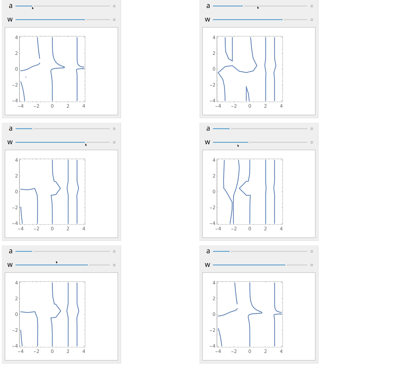
enter image description here

If you want to extract the lines from a given value of a and w you can right click the plot and copy it and then paste into a new cell and use :

template of code below : points = Cases[Normal[... plot here ...], Line[x_] :> x, All]
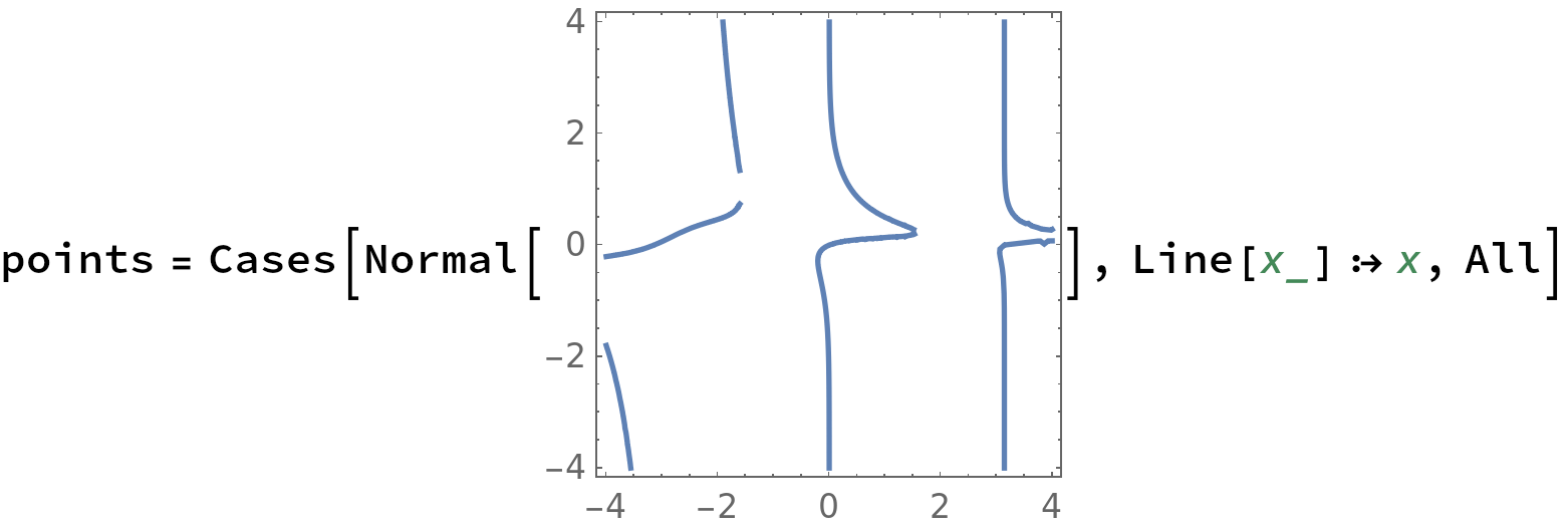
enter image description here

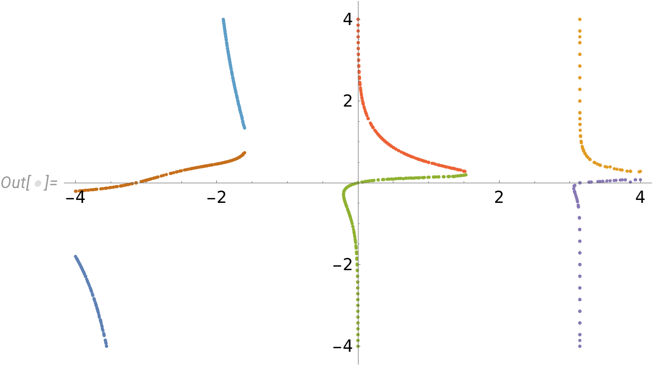
The points:

points // ListPlot

enter image description here


enter image description here

The points above might not be very accurate. In that case consider the numerical methods here: How to find seed values for solving nonlinear equations?

expression = (a b A Exp[-b (x - a)])/(a Exp[-b (x - a)] + 1)^2 + 
  c Tan[x]

$$ \frac{a A b e^{-b (x-a)}}{\left(a e^{-b (x-a)}+1\right)^2}+c \tan (x) $$


For non zero c, we can absorb the dependence on c by dividing by c and using A->c*w :

expression2 = expression/c /. A -> w*c // Simplify

$$\frac{a b w e^{b (x-a)}}{\left(e^{b (x-a)}+a\right)^2}+\tan (x)$$

That way there is one less parameter to consider but do not forget to check separately the case c=0. In the following I will focus on c non zero.

For generic parameters Mathematica can not find a root for expression. However, it can find instances of roots using FindInstance. For example, if we consider a to be positive then :

FindInstance[{expression2 == 0, a > 0}, {x, a, b, w}]

{{x->9392403/3312026,a->26566113/18118801,b->30971405/14149612,w->-((256374004055212 (26566113/18118801+E^(2545583876943569930325/849117367154967579512))^2 Tan[9392403/3312026])/(822789844998765 E^(2545583876943569930325/849117367154967579512)))}}

We can visualize dependence on parameters using (recall that c=0 should be considered separately):

Note: I chose the ranges of parameters in an arbitrary manner

  With[{expression2 = expression2}, 
 Manipulate[
  ContourPlot[expression2 == 0, {x, -4, 4}, {b, -4, 4}], {a, -4, 
   4}, {w, -4, 4}]]

enter image description here

If you want to extract the lines from a given value of a and w you can right click the plot and copy it and then paste into a new cell and use :

template of code below : points = Cases[Normal[... plot here ...], Line[x_] :> x, All]

enter image description here

The points:

points // ListPlot

enter image description here


The points above might not be very accurate. In that case consider the numerical methods here: How to find seed values for solving nonlinear equations?

expression = (a b A Exp[-b (x - a)])/(a Exp[-b (x - a)] + 1)^2 + 
  c Tan[x]

$$ \frac{a A b e^{-b (x-a)}}{\left(a e^{-b (x-a)}+1\right)^2}+c \tan (x) $$


For non zero c, we can absorb the dependence on c by dividing by c and using A->c*w :

expression2 = expression/c /. A -> w*c // Simplify

$$\frac{a b w e^{b (x-a)}}{\left(e^{b (x-a)}+a\right)^2}+\tan (x)$$

That way there is one less parameter to consider but do not forget to check separately the case c=0. In the following I will focus on c non zero.

For generic parameters Mathematica can not find a root for expression above. However, it can find instances of roots using FindInstance. For example, if we consider a to be positive then :

FindInstance[{expression2 == 0, a > 0}, {x, a, b, w}]

{{x->9392403/3312026,a->26566113/18118801,b->30971405/14149612,w->-((256374004055212 (26566113/18118801+E^(2545583876943569930325/849117367154967579512))^2 Tan[9392403/3312026])/(822789844998765 E^(2545583876943569930325/849117367154967579512)))}}

We can visualize dependence on parameters using (recall that c=0 should be considered separately):

Note: I chose the ranges of parameters in an arbitrary manner

  With[{expression2 = expression2}, 
 Manipulate[
  ContourPlot[expression2 == 0, {x, -4, 4}, {b, -4, 4}], {a, -4, 
   4}, {w, -4, 4}]]

enter image description here

If you want to extract the lines from a given value of a and w you can right click the plot and copy it and then paste into a new cell and use :

template of code below : points = Cases[Normal[... plot here ...], Line[x_] :> x, All]

enter image description here

The points:

points // ListPlot

enter image description here

The points above might not be very accurate. In that case consider the numerical methods here: How to find seed values for solving nonlinear equations?

added 74 characters in body
Source Link
Loading
Source Link
Loading