added 5 characters in body
Source Link
Yaroslav Bulatov
  • 6.7k
  • 1
  • 21
  • 47

I need to randomlyisotropically sample vectors in $\mathbb{R}^d$ of Euclidean norm $c$ such that components are positive and add up to 1. Any suggestions how to do this in Mathematica?

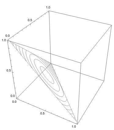
For $d=3$ this means sampling from one of the circular contours in

SliceContourPlot3D[Sqrt[x^2 + y^2 + z^2], 
 x + y + z == 1, {x, 0, 1}, {y, 0, 1}, {z, 0, 1}]

enter image description here

Things I tried

  1. RandomPoint[ RegionIntersection[Sphere[{0, 0, 0}, .9], Simplex[IdentityMatrix[3]]]] -- returns unevaluated
  2. Rejection sampling. Inefficient for $d=3$, completely impractical for higher values, I need $d=100$.

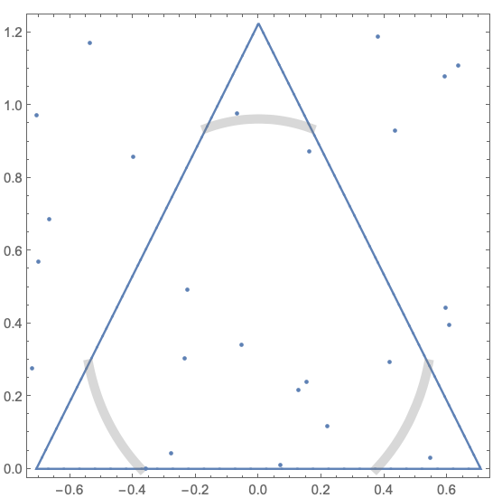
Code below is for debugging rejection sampling in $d=3$ case. It takes a sample of 3d points, projects onto $x_1+x_2+x_3=1$ plane, displays them along with the target region marked in gray. Will appreciate any suggestions on making an efficient sampler.

enter image description here


(* simplex visualization code from https://mathematica.stackexchange.com/a/139443/217 *)
visualize[points_, c_] := Module[{},
   d = 3;
   kk = Array[k, 6];
   mat = Partition[kk, 2];
   bb = Array[b, 3];
   source = {{-1/Sqrt[2], 0}, {1/Sqrt[2], 0}, {0, Sqrt[3/2]}};
   target = IdentityMatrix[3];
   eqs = Table[mat . source[[i]] + bb == target[[i]], {i, 3}]; 
   sol = First@Solve[eqs, kk~Join~bb];
   {mat0, bb0} = {mat, bb} /. sol;
   imat0 = PseudoInverse[mat0];
   unmap[point_] := imat0 . (point - bb0);
   expr = mat0 . {x, y} + bb0;
   reg = ImplicitRegion[Reduce[Thread[expr > 0]], {x, y}];
   
   regionPlot = RegionPlot[reg, PlotStyle -> None];
   pointsPlot = ListPlot[unmap /@ points];
   val = Sqrt[Total[expr^2]];
   contourPlot = 
    ContourPlot[val == c, {x, y} \[Element] reg, 
     AspectRatio -> Automatic, PlotPoints -> 10, 
     ContourShading -> None, 
     ContourStyle -> Directive[Opacity[.3], Gray, Thickness[.02]]];
   
   Show[regionPlot, contourPlot, pointsPlot]
   ];

points = RandomVariate[NormalDistribution[], {100, 3}];
visualize[points, .8]

Motivation is to get a diverse sampling of discrete distributions of given complexity. JimB's previous answer achieves some progress for the case when entropy is the complexity measure. This question corresponds to linear entropy as the complexity measure. Related question on math.SE.

I need to randomly sample vectors in $\mathbb{R}^d$ of Euclidean norm $c$ such that components are positive and add up to 1. Any suggestions how to do this in Mathematica?

For $d=3$ this means sampling from one of the circular contours in

SliceContourPlot3D[Sqrt[x^2 + y^2 + z^2], 
 x + y + z == 1, {x, 0, 1}, {y, 0, 1}, {z, 0, 1}]

enter image description here

Things I tried

  1. RandomPoint[ RegionIntersection[Sphere[{0, 0, 0}, .9], Simplex[IdentityMatrix[3]]]] -- returns unevaluated
  2. Rejection sampling. Inefficient for $d=3$, completely impractical for higher values, I need $d=100$.

Code below is for debugging rejection sampling in $d=3$ case. It takes a sample of 3d points, projects onto $x_1+x_2+x_3=1$ plane, displays them along with the target region marked in gray. Will appreciate any suggestions on making an efficient sampler.

enter image description here


(* simplex visualization code from https://mathematica.stackexchange.com/a/139443/217 *)
visualize[points_, c_] := Module[{},
   d = 3;
   kk = Array[k, 6];
   mat = Partition[kk, 2];
   bb = Array[b, 3];
   source = {{-1/Sqrt[2], 0}, {1/Sqrt[2], 0}, {0, Sqrt[3/2]}};
   target = IdentityMatrix[3];
   eqs = Table[mat . source[[i]] + bb == target[[i]], {i, 3}]; 
   sol = First@Solve[eqs, kk~Join~bb];
   {mat0, bb0} = {mat, bb} /. sol;
   imat0 = PseudoInverse[mat0];
   unmap[point_] := imat0 . (point - bb0);
   expr = mat0 . {x, y} + bb0;
   reg = ImplicitRegion[Reduce[Thread[expr > 0]], {x, y}];
   
   regionPlot = RegionPlot[reg, PlotStyle -> None];
   pointsPlot = ListPlot[unmap /@ points];
   val = Sqrt[Total[expr^2]];
   contourPlot = 
    ContourPlot[val == c, {x, y} \[Element] reg, 
     AspectRatio -> Automatic, PlotPoints -> 10, 
     ContourShading -> None, 
     ContourStyle -> Directive[Opacity[.3], Gray, Thickness[.02]]];
   
   Show[regionPlot, contourPlot, pointsPlot]
   ];

points = RandomVariate[NormalDistribution[], {100, 3}];
visualize[points, .8]

Motivation is to get a diverse sampling of discrete distributions of given complexity. JimB's previous answer achieves some progress for the case when entropy is the complexity measure. This question corresponds to linear entropy as the complexity measure. Related question on math.SE.
I need to isotropically sample vectors in $\mathbb{R}^d$ of Euclidean norm $c$ such that components are positive and add up to 1. Any suggestions how to do this in Mathematica?

For $d=3$ this means sampling from one of the circular contours in

SliceContourPlot3D[Sqrt[x^2 + y^2 + z^2], 
 x + y + z == 1, {x, 0, 1}, {y, 0, 1}, {z, 0, 1}]

enter image description here

Things I tried

  1. RandomPoint[ RegionIntersection[Sphere[{0, 0, 0}, .9], Simplex[IdentityMatrix[3]]]] -- returns unevaluated
  2. Rejection sampling. Inefficient for $d=3$, completely impractical for higher values, I need $d=100$.

Code below is for debugging rejection sampling in $d=3$ case. It takes a sample of 3d points, projects onto $x_1+x_2+x_3=1$ plane, displays them along with the target region marked in gray. Will appreciate any suggestions on making an efficient sampler.

enter image description here


(* simplex visualization code from https://mathematica.stackexchange.com/a/139443/217 *)
visualize[points_, c_] := Module[{},
   d = 3;
   kk = Array[k, 6];
   mat = Partition[kk, 2];
   bb = Array[b, 3];
   source = {{-1/Sqrt[2], 0}, {1/Sqrt[2], 0}, {0, Sqrt[3/2]}};
   target = IdentityMatrix[3];
   eqs = Table[mat . source[[i]] + bb == target[[i]], {i, 3}]; 
   sol = First@Solve[eqs, kk~Join~bb];
   {mat0, bb0} = {mat, bb} /. sol;
   imat0 = PseudoInverse[mat0];
   unmap[point_] := imat0 . (point - bb0);
   expr = mat0 . {x, y} + bb0;
   reg = ImplicitRegion[Reduce[Thread[expr > 0]], {x, y}];
   
   regionPlot = RegionPlot[reg, PlotStyle -> None];
   pointsPlot = ListPlot[unmap /@ points];
   val = Sqrt[Total[expr^2]];
   contourPlot = 
    ContourPlot[val == c, {x, y} \[Element] reg, 
     AspectRatio -> Automatic, PlotPoints -> 10, 
     ContourShading -> None, 
     ContourStyle -> Directive[Opacity[.3], Gray, Thickness[.02]]];
   
   Show[regionPlot, contourPlot, pointsPlot]
   ];

points = RandomVariate[NormalDistribution[], {100, 3}];
visualize[points, .8]

Motivation is to get a diverse sampling of discrete distributions of given complexity. JimB's previous answer achieves some progress for the case when entropy is the complexity measure. This question corresponds to linear entropy as the complexity measure. Related question on math.SE.

Became Hot Network Question
Tweeted twitter.com/StackMma/status/1571604981471387659
deleted 4 characters in body
Source Link
Yaroslav Bulatov
  • 6.7k
  • 1
  • 21
  • 47

I need to randomly sample vectors in $\mathbb{R}^d$ of Euclidean norm $c$ such that components are positive and add up to 1. Any suggestions how to do this in Mathematica?

For $d=3$ this means sampling from one of the circular contours in

SliceContourPlot3D[Sqrt[x^2 + y^2 + z^2], 
 x + y + z == 1, {x, 0, 1}, {y, 0, 1}, {z, 0, 1}]

enter image description here

Things I tried

  1. RandomPoint[ RegionIntersection[Sphere[{0, 0, 0}, .9], Simplex[IdentityMatrix[3]]]] -- returns unevaluated
  2. Rejection sampling. Inefficient for $d=3$, completely impractical for higher values, I need $d=100$.

Code below is for debugging rejection sampling in $d=3$ case. It takes a sample of 3d points, projects onto $x_1+x_2+x_3=1$ plane, displays them along with the target region marked in gray. Will appreciate any suggestions on making a morean efficient sampler.

enter image description here


(* simplex visualization code from https://mathematica.stackexchange.com/a/139443/217 *)
visualize[points_, c_] := Module[{},
   d = 3;
   kk = Array[k, 6];
   mat = Partition[kk, 2];
   bb = Array[b, 3];
   source = {{-1/Sqrt[2], 0}, {1/Sqrt[2], 0}, {0, Sqrt[3/2]}};
   target = IdentityMatrix[3];
   eqs = Table[mat . source[[i]] + bb == target[[i]], {i, 3}]; 
   sol = First@Solve[eqs, kk~Join~bb];
   {mat0, bb0} = {mat, bb} /. sol;
   imat0 = PseudoInverse[mat0];
   unmap[point_] := imat0 . (point - bb0);
   expr = mat0 . {x, y} + bb0;
   reg = ImplicitRegion[Reduce[Thread[expr > 0]], {x, y}];
   
   regionPlot = RegionPlot[reg, PlotStyle -> None];
   pointsPlot = ListPlot[unmap /@ points];
   val = Sqrt[Total[expr^2]];
   contourPlot = 
    ContourPlot[val == c, {x, y} \[Element] reg, 
     AspectRatio -> Automatic, PlotPoints -> 10, 
     ContourShading -> None, 
     ContourStyle -> Directive[Opacity[.3], Gray, Thickness[.02]]];
   
   Show[regionPlot, contourPlot, pointsPlot]
   ];

points = RandomVariate[NormalDistribution[], {100, 3}];
visualize[points, .8]

Motivation is to get a diverse sampling of discrete distributions of given complexity. JimB's previous answer achieves some progress for the case when entropy is the complexity measure. This question corresponds to linear entropy as the complexity measure. Related question on math.SE.

I need to randomly sample vectors in $\mathbb{R}^d$ of Euclidean norm $c$ such that components are positive and add up to 1. Any suggestions how to do this in Mathematica?

For $d=3$ this means sampling from one of the circular contours in

SliceContourPlot3D[Sqrt[x^2 + y^2 + z^2], 
 x + y + z == 1, {x, 0, 1}, {y, 0, 1}, {z, 0, 1}]

enter image description here

Things I tried

  1. RandomPoint[ RegionIntersection[Sphere[{0, 0, 0}, .9], Simplex[IdentityMatrix[3]]]] -- returns unevaluated
  2. Rejection sampling. Inefficient for $d=3$, completely impractical for higher values, I need $d=100$.

Code below is for debugging rejection sampling in $d=3$ case. It takes a sample of 3d points, projects onto $x_1+x_2+x_3=1$ plane, displays them along with the target region marked in gray. Will appreciate any suggestions on making a more efficient sampler.

enter image description here


(* simplex visualization code from https://mathematica.stackexchange.com/a/139443/217 *)
visualize[points_, c_] := Module[{},
   d = 3;
   kk = Array[k, 6];
   mat = Partition[kk, 2];
   bb = Array[b, 3];
   source = {{-1/Sqrt[2], 0}, {1/Sqrt[2], 0}, {0, Sqrt[3/2]}};
   target = IdentityMatrix[3];
   eqs = Table[mat . source[[i]] + bb == target[[i]], {i, 3}]; 
   sol = First@Solve[eqs, kk~Join~bb];
   {mat0, bb0} = {mat, bb} /. sol;
   imat0 = PseudoInverse[mat0];
   unmap[point_] := imat0 . (point - bb0);
   expr = mat0 . {x, y} + bb0;
   reg = ImplicitRegion[Reduce[Thread[expr > 0]], {x, y}];
   
   regionPlot = RegionPlot[reg, PlotStyle -> None];
   pointsPlot = ListPlot[unmap /@ points];
   val = Sqrt[Total[expr^2]];
   contourPlot = 
    ContourPlot[val == c, {x, y} \[Element] reg, 
     AspectRatio -> Automatic, PlotPoints -> 10, 
     ContourShading -> None, 
     ContourStyle -> Directive[Opacity[.3], Gray, Thickness[.02]]];
   
   Show[regionPlot, contourPlot, pointsPlot]
   ];

points = RandomVariate[NormalDistribution[], {100, 3}];
visualize[points, .8]

Motivation is to get a diverse sampling of discrete distributions of given complexity. JimB's previous answer achieves some progress for the case when entropy is the complexity measure. This question corresponds to linear entropy as the complexity measure. Related question on math.SE.

I need to randomly sample vectors in $\mathbb{R}^d$ of Euclidean norm $c$ such that components are positive and add up to 1. Any suggestions how to do this in Mathematica?

For $d=3$ this means sampling from one of the circular contours in

SliceContourPlot3D[Sqrt[x^2 + y^2 + z^2], 
 x + y + z == 1, {x, 0, 1}, {y, 0, 1}, {z, 0, 1}]

enter image description here

Things I tried

  1. RandomPoint[ RegionIntersection[Sphere[{0, 0, 0}, .9], Simplex[IdentityMatrix[3]]]] -- returns unevaluated
  2. Rejection sampling. Inefficient for $d=3$, completely impractical for higher values, I need $d=100$.

Code below is for debugging rejection sampling in $d=3$ case. It takes a sample of 3d points, projects onto $x_1+x_2+x_3=1$ plane, displays them along with the target region marked in gray. Will appreciate any suggestions on making an efficient sampler.

enter image description here


(* simplex visualization code from https://mathematica.stackexchange.com/a/139443/217 *)
visualize[points_, c_] := Module[{},
   d = 3;
   kk = Array[k, 6];
   mat = Partition[kk, 2];
   bb = Array[b, 3];
   source = {{-1/Sqrt[2], 0}, {1/Sqrt[2], 0}, {0, Sqrt[3/2]}};
   target = IdentityMatrix[3];
   eqs = Table[mat . source[[i]] + bb == target[[i]], {i, 3}]; 
   sol = First@Solve[eqs, kk~Join~bb];
   {mat0, bb0} = {mat, bb} /. sol;
   imat0 = PseudoInverse[mat0];
   unmap[point_] := imat0 . (point - bb0);
   expr = mat0 . {x, y} + bb0;
   reg = ImplicitRegion[Reduce[Thread[expr > 0]], {x, y}];
   
   regionPlot = RegionPlot[reg, PlotStyle -> None];
   pointsPlot = ListPlot[unmap /@ points];
   val = Sqrt[Total[expr^2]];
   contourPlot = 
    ContourPlot[val == c, {x, y} \[Element] reg, 
     AspectRatio -> Automatic, PlotPoints -> 10, 
     ContourShading -> None, 
     ContourStyle -> Directive[Opacity[.3], Gray, Thickness[.02]]];
   
   Show[regionPlot, contourPlot, pointsPlot]
   ];

points = RandomVariate[NormalDistribution[], {100, 3}];
visualize[points, .8]

Motivation is to get a diverse sampling of discrete distributions of given complexity. JimB's previous answer achieves some progress for the case when entropy is the complexity measure. This question corresponds to linear entropy as the complexity measure. Related question on math.SE.

added 9 characters in body
Source Link
Yaroslav Bulatov
  • 6.7k
  • 1
  • 21
  • 47

I need to randomly sample vectors in $\mathbb{R}^d$ of Euclidean norm $c$ such that components are positive and add up to 1. Any suggestions how to do this in Mathematica?

For $d=3$ this means sampling from one of the circular contours in

SliceContourPlot3D[Sqrt[x^2 + y^2 + z^2], 
 x + y + z == 1, {x, 0, 1}, {y, 0, 1}, {z, 0, 1}]

enter image description here

Things I tried

  1. RandomPoint[ RegionIntersection[Sphere[{0, 0, 0}, .9], Simplex[IdentityMatrix[3]]]] -- returns unevaluated
  2. Rejection sampling. Inefficient for $d=3$, completely impractical for higher values, I need $d=100$.

Code below is for debugging rejection sampling in $d=3$ case. VisualizeIt takes a sample of 3d points, projects onto $x_1+x_2+x_3=1$ plane, displays them along with the target region marked in gray. Will appreciate any suggestions on making a usablemore efficient sampler for $d=100$.

enter image description here


(* simplex visualization code from https://mathematica.stackexchange.com/a/139443/217 *)
visualize[points_, c_] := Module[{},
   d = 3;
   kk = Array[k, 6];
   mat = Partition[kk, 2];
   bb = Array[b, 3];
   source = {{-1/Sqrt[2], 0}, {1/Sqrt[2], 0}, {0, Sqrt[3/2]}};
   target = IdentityMatrix[3];
   eqs = Table[mat . source[[i]] + bb == target[[i]], {i, 3}]; 
   sol = First@Solve[eqs, kk~Join~bb];
   {mat0, bb0} = {mat, bb} /. sol;
   imat0 = PseudoInverse[mat0];
   unmap[point_] := imat0 . (point - bb0);
   expr = mat0 . {x, y} + bb0;
   reg = ImplicitRegion[Reduce[Thread[expr > 0]], {x, y}];
   
   regionPlot = RegionPlot[reg, PlotStyle -> None];
   pointsPlot = ListPlot[unmap /@ points];
   val = Sqrt[Total[expr^2]];
   contourPlot = 
    ContourPlot[val == c, {x, y} \[Element] reg, 
     AspectRatio -> Automatic, PlotPoints -> 10, 
     ContourShading -> None, 
     ContourStyle -> Directive[Opacity[.3], Gray, Thickness[.02]]];
   
   Show[regionPlot, contourPlot, pointsPlot]
   ];

points = RandomVariate[NormalDistribution[], {100, 3}];
visualize[points, .8]

Motivation is to sampleget a diverse sampling of discrete distributions of given complexity. JimB's previous answer achieves some progress for the case when entropy is the complexity measure. This question corresponds to linear entropy as the complexity measure. Related question on math.SE.

I need to randomly sample vectors in $\mathbb{R}^d$ of Euclidean norm $c$ such that components are positive and add up to 1. Any suggestions how to do this in Mathematica?

For $d=3$ this means sampling from one of the circular contours in

SliceContourPlot3D[Sqrt[x^2 + y^2 + z^2], 
 x + y + z == 1, {x, 0, 1}, {y, 0, 1}, {z, 0, 1}]

enter image description here

Things I tried

  1. RandomPoint[ RegionIntersection[Sphere[{0, 0, 0}, .9], Simplex[IdentityMatrix[3]]]] -- returns unevaluated
  2. Rejection sampling. Inefficient for $d=3$, completely impractical for higher values, I need $d=100$.

Code below is for debugging $d=3$ case. Visualize a sample of points along with the target region marked in gray. Will appreciate any suggestions on making a usable sampler for $d=100$.

enter image description here


(* simplex visualization code from https://mathematica.stackexchange.com/a/139443/217 *)
visualize[points_, c_] := Module[{},
   d = 3;
   kk = Array[k, 6];
   mat = Partition[kk, 2];
   bb = Array[b, 3];
   source = {{-1/Sqrt[2], 0}, {1/Sqrt[2], 0}, {0, Sqrt[3/2]}};
   target = IdentityMatrix[3];
   eqs = Table[mat . source[[i]] + bb == target[[i]], {i, 3}]; 
   sol = First@Solve[eqs, kk~Join~bb];
   {mat0, bb0} = {mat, bb} /. sol;
   imat0 = PseudoInverse[mat0];
   unmap[point_] := imat0 . (point - bb0);
   expr = mat0 . {x, y} + bb0;
   reg = ImplicitRegion[Reduce[Thread[expr > 0]], {x, y}];
   
   regionPlot = RegionPlot[reg, PlotStyle -> None];
   pointsPlot = ListPlot[unmap /@ points];
   val = Sqrt[Total[expr^2]];
   contourPlot = 
    ContourPlot[val == c, {x, y} \[Element] reg, 
     AspectRatio -> Automatic, PlotPoints -> 10, 
     ContourShading -> None, 
     ContourStyle -> Directive[Opacity[.3], Gray, Thickness[.02]]];
   
   Show[regionPlot, contourPlot, pointsPlot]
   ];

points = RandomVariate[NormalDistribution[], {100, 3}];
visualize[points, .8]

Motivation is to sample discrete distributions of given complexity. JimB's previous answer achieves some progress for the case when entropy is the complexity measure. This question corresponds to linear entropy as the complexity measure. Related question on math.SE.

I need to randomly sample vectors in $\mathbb{R}^d$ of Euclidean norm $c$ such that components are positive and add up to 1. Any suggestions how to do this in Mathematica?

For $d=3$ this means sampling from one of the circular contours in

SliceContourPlot3D[Sqrt[x^2 + y^2 + z^2], 
 x + y + z == 1, {x, 0, 1}, {y, 0, 1}, {z, 0, 1}]

enter image description here

Things I tried

  1. RandomPoint[ RegionIntersection[Sphere[{0, 0, 0}, .9], Simplex[IdentityMatrix[3]]]] -- returns unevaluated
  2. Rejection sampling. Inefficient for $d=3$, completely impractical for higher values, I need $d=100$.

Code below is for debugging rejection sampling in $d=3$ case. It takes a sample of 3d points, projects onto $x_1+x_2+x_3=1$ plane, displays them along with the target region marked in gray. Will appreciate any suggestions on making a more efficient sampler.

enter image description here


(* simplex visualization code from https://mathematica.stackexchange.com/a/139443/217 *)
visualize[points_, c_] := Module[{},
   d = 3;
   kk = Array[k, 6];
   mat = Partition[kk, 2];
   bb = Array[b, 3];
   source = {{-1/Sqrt[2], 0}, {1/Sqrt[2], 0}, {0, Sqrt[3/2]}};
   target = IdentityMatrix[3];
   eqs = Table[mat . source[[i]] + bb == target[[i]], {i, 3}]; 
   sol = First@Solve[eqs, kk~Join~bb];
   {mat0, bb0} = {mat, bb} /. sol;
   imat0 = PseudoInverse[mat0];
   unmap[point_] := imat0 . (point - bb0);
   expr = mat0 . {x, y} + bb0;
   reg = ImplicitRegion[Reduce[Thread[expr > 0]], {x, y}];
   
   regionPlot = RegionPlot[reg, PlotStyle -> None];
   pointsPlot = ListPlot[unmap /@ points];
   val = Sqrt[Total[expr^2]];
   contourPlot = 
    ContourPlot[val == c, {x, y} \[Element] reg, 
     AspectRatio -> Automatic, PlotPoints -> 10, 
     ContourShading -> None, 
     ContourStyle -> Directive[Opacity[.3], Gray, Thickness[.02]]];
   
   Show[regionPlot, contourPlot, pointsPlot]
   ];

points = RandomVariate[NormalDistribution[], {100, 3}];
visualize[points, .8]

Motivation is to get a diverse sampling of discrete distributions of given complexity. JimB's previous answer achieves some progress for the case when entropy is the complexity measure. This question corresponds to linear entropy as the complexity measure. Related question on math.SE.

added 9 characters in body
Source Link
Yaroslav Bulatov
  • 6.7k
  • 1
  • 21
  • 47
Loading
Source Link
Yaroslav Bulatov
  • 6.7k
  • 1
  • 21
  • 47
Loading