added 1610 characters in body
Source Link
Alex Trounev
  • 48.8k
  • 3
  • 51
  • 115

To solve the problem of broken lines we can use hand made code. First, we define interpolation functions for $B_x,B_z$ to exclude singularities as follows

Bx = Interpolation[
  Flatten[Table[{x, 
     z, \[ScriptCapitalB]BarMagnet[{x, 0., z}, {1.5, .5, 
        5.5}] [[1]]}, {x, 0, 10, .1}, {z, 0, 10, .1}], 1]];

Bz = Interpolation[
  Flatten[Table[{x, 
     z, \[ScriptCapitalB]BarMagnet[{x, 0., z}, {1.5, .5, 
        5.5}] [[3]]}, {x, 0, 10, .1}, {z, 0, 10, .1}], 1]];

Second, we compute field lines with

X1 = ParametricNDSolveValue[{z'[t] == Bz[x[t], z[t]], 
   x'[t] == Bx[x[t], z[t]], x[0] == x0, z[0] == z0}, 
  x, {t, 0, 1000}, {x0, z0}]; 
Z1 = 
     ParametricNDSolveValue[{x'[t] == Bx[x[t], z[t]], 
       z'[t] == Bz[x[t], z[t]], x[0] == x0, z[0] == z0}, 
      z, {t, 0, 1000}, {x0, z0}]; 

Finally we plot stream lines with StreamPlot[] and ParametricPlot[], and show in one plot

sp = StreamPlot[{Bx[x, z], Bz[x, z]} ,   {x, 0, 10}, {z, 0, 10}, 
                              PlotRange -> All,
                                StreamPoints -> Fine, 
  AspectRatio -> Automatic, Frame -> None, 
  StreamColorFunction -> "Rainbow", StreamScale -> None, 
  VectorPoints -> Fine, PerformanceGoal -> "Quality", 
  MaxRecursion -> 2];
ppxz = ParametricPlot[
   Table[{X1[x0, 0.01][t], Z1[x0, 0.01][t]}, {x0, .1, .5, .1}], {t, 0,
     1000}, PlotStyle -> Red];

Show[sp, ppxz]

Figure 2

To solve the problem of broken lines we can use hand made code. First, we define interpolation functions for $B_x,B_z$ to exclude singularities as follows

Bx = Interpolation[
  Flatten[Table[{x, 
     z, \[ScriptCapitalB]BarMagnet[{x, 0., z}, {1.5, .5, 
        5.5}] [[1]]}, {x, 0, 10, .1}, {z, 0, 10, .1}], 1]];

Bz = Interpolation[
  Flatten[Table[{x, 
     z, \[ScriptCapitalB]BarMagnet[{x, 0., z}, {1.5, .5, 
        5.5}] [[3]]}, {x, 0, 10, .1}, {z, 0, 10, .1}], 1]];

Second, we compute field lines with

X1 = ParametricNDSolveValue[{z'[t] == Bz[x[t], z[t]], 
   x'[t] == Bx[x[t], z[t]], x[0] == x0, z[0] == z0}, 
  x, {t, 0, 1000}, {x0, z0}]; 
Z1 = 
     ParametricNDSolveValue[{x'[t] == Bx[x[t], z[t]], 
       z'[t] == Bz[x[t], z[t]], x[0] == x0, z[0] == z0}, 
      z, {t, 0, 1000}, {x0, z0}]; 

Finally we plot stream lines with StreamPlot[] and ParametricPlot[], and show in one plot

sp = StreamPlot[{Bx[x, z], Bz[x, z]} ,   {x, 0, 10}, {z, 0, 10}, 
                              PlotRange -> All,
                                StreamPoints -> Fine, 
  AspectRatio -> Automatic, Frame -> None, 
  StreamColorFunction -> "Rainbow", StreamScale -> None, 
  VectorPoints -> Fine, PerformanceGoal -> "Quality", 
  MaxRecursion -> 2];
ppxz = ParametricPlot[
   Table[{X1[x0, 0.01][t], Z1[x0, 0.01][t]}, {x0, .1, .5, .1}], {t, 0,
     1000}, PlotStyle -> Red];

Show[sp, ppxz]
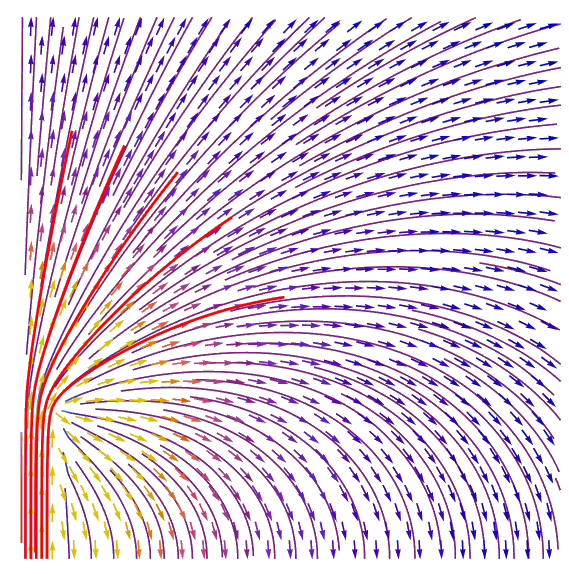
Figure 2

added 173 characters in body
Source Link
Alex Trounev
  • 48.8k
  • 3
  • 51
  • 115

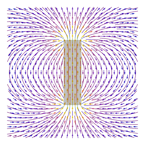
To show continues field line we use option StreamScale -> None

\[Psi]BarMagnetHeld  = 
  WolframAlpha[
   "magnetic potential rectangular bar magnet", {{"Result", 1}, 
    "Input"}];
\[Psi]BarMagnet[{x_, y_, z_}, {a_, b_, 
    c_}] = (ReleaseHold[\[Psi]BarMagnetHeld] /. {QuantityVariable[x_, 
        y_] :> x})/Subscript[M, 0];
\[ScriptCapitalH]BarMagnet[{x_, y_, z_}, {a_, b_, 
    c_}] = -D[\[Psi]BarMagnet[{x, y, z}, {a, b, c}], {{x, y, z}}];
\[ScriptCapitalB]BarMagnet[{x_, y_, z_}, {a_, b_, 
    c_}] = \[ScriptCapitalH]BarMagnet[{x, y, z}, {a, b, c}] + {0, 0, 
     1} UnitStep[(a/2)^2 - x^2] UnitStep[(b/2)^2 - 
      y^2] UnitStep[(c/2)^2 - z^2];

crossSectionFieldPlot[field_, fieldStrength_] := 
 Block[{a = 1.5, b = 0.5, c = 5.5},
    StreamPlot[fieldStrength ,   {x, -c/2, c/2}, {z, -.75 c, .75 c}, 
                               PlotRange -> All,
                                 StreamPoints -> Fine, 
   AspectRatio -> Automatic, Frame -> None, 
   StreamColorFunction -> "Rainbow"]"Rainbow", StreamScale -> None, 
   VectorPoints -> Fine, PerformanceGoal -> "Quality", 
   MaxRecursion -> 10]
  ]
bar2 = With[{a = 1.5,  c = 5.5}, 
  Graphics[{Opacity[.25], Rectangle[{-a, -c}/2, {a, c}/2]}, 
   Axes -> False, Frame -> False]]False]];
Show[crossSectionFieldPlot[
  "\[ScriptCapitalB]", \[ScriptCapitalB]BarMagnet[{x, 0, z}, {a, b, 
     c}] [[{1, 3}]]] , bar2] 

Figure 1Figure 1

\[Psi]BarMagnetHeld  = 
  WolframAlpha[
   "magnetic potential rectangular bar magnet", {{"Result", 1}, 
    "Input"}];
\[Psi]BarMagnet[{x_, y_, z_}, {a_, b_, 
    c_}] = (ReleaseHold[\[Psi]BarMagnetHeld] /. {QuantityVariable[x_, 
        y_] :> x})/Subscript[M, 0];
\[ScriptCapitalH]BarMagnet[{x_, y_, z_}, {a_, b_, 
    c_}] = -D[\[Psi]BarMagnet[{x, y, z}, {a, b, c}], {{x, y, z}}];
\[ScriptCapitalB]BarMagnet[{x_, y_, z_}, {a_, b_, 
    c_}] = \[ScriptCapitalH]BarMagnet[{x, y, z}, {a, b, c}] + {0, 0, 
     1} UnitStep[(a/2)^2 - x^2] UnitStep[(b/2)^2 - 
      y^2] UnitStep[(c/2)^2 - z^2];

crossSectionFieldPlot[field_, fieldStrength_] := 
 Block[{a = 1.5, b = 0.5, c = 5.5},
    StreamPlot[fieldStrength ,   {x, -c/2, c/2}, {z, -.75 c, .75 c}, 
                               PlotRange -> All,
                                 StreamPoints -> Fine, 
   AspectRatio -> Automatic, Frame -> None, 
   StreamColorFunction -> "Rainbow"]
  ]
bar2 = With[{a = 1.5,  c = 5.5}, 
  Graphics[{Opacity[.25], Rectangle[{-a, -c}/2, {a, c}/2]}, 
   Axes -> False, Frame -> False]]
Show[crossSectionFieldPlot[
  "\[ScriptCapitalB]", \[ScriptCapitalB]BarMagnet[{x, 0, z}, {a, b, 
     c}] [[{1, 3}]]] , bar2]

Figure 1

To show continues field line we use option StreamScale -> None

\[Psi]BarMagnetHeld  = 
  WolframAlpha[
   "magnetic potential rectangular bar magnet", {{"Result", 1}, 
    "Input"}];
\[Psi]BarMagnet[{x_, y_, z_}, {a_, b_, 
    c_}] = (ReleaseHold[\[Psi]BarMagnetHeld] /. {QuantityVariable[x_, 
        y_] :> x})/Subscript[M, 0];
\[ScriptCapitalH]BarMagnet[{x_, y_, z_}, {a_, b_, 
    c_}] = -D[\[Psi]BarMagnet[{x, y, z}, {a, b, c}], {{x, y, z}}];
\[ScriptCapitalB]BarMagnet[{x_, y_, z_}, {a_, b_, 
    c_}] = \[ScriptCapitalH]BarMagnet[{x, y, z}, {a, b, c}] + {0, 0, 
     1} UnitStep[(a/2)^2 - x^2] UnitStep[(b/2)^2 - 
      y^2] UnitStep[(c/2)^2 - z^2];

crossSectionFieldPlot[field_, fieldStrength_] := 
 Block[{a = 1.5, b = 0.5, c = 5.5},
    StreamPlot[fieldStrength ,   {x, -c, c}, {z, -c, c}, 
                               PlotRange -> All,
                                 StreamPoints -> Fine, 
   AspectRatio -> Automatic, Frame -> None, 
   StreamColorFunction -> "Rainbow", StreamScale -> None, 
   VectorPoints -> Fine, PerformanceGoal -> "Quality", 
   MaxRecursion -> 10]
  ]
bar2 = With[{a = 1.5,  c = 5.5}, 
  Graphics[{Opacity[.25], Rectangle[{-a, -c}/2, {a, c}/2]}, 
   Axes -> False, Frame -> False]];
Show[crossSectionFieldPlot[
  "\[ScriptCapitalB]", \[ScriptCapitalB]BarMagnet[{x, 0, z}, {a, b, 
     c}] [[{1, 3}]]] , bar2] 

Figure 1

Source Link
Alex Trounev
  • 48.8k
  • 3
  • 51
  • 115

\[Psi]BarMagnetHeld  = 
  WolframAlpha[
   "magnetic potential rectangular bar magnet", {{"Result", 1}, 
    "Input"}];
\[Psi]BarMagnet[{x_, y_, z_}, {a_, b_, 
    c_}] = (ReleaseHold[\[Psi]BarMagnetHeld] /. {QuantityVariable[x_, 
        y_] :> x})/Subscript[M, 0];
\[ScriptCapitalH]BarMagnet[{x_, y_, z_}, {a_, b_, 
    c_}] = -D[\[Psi]BarMagnet[{x, y, z}, {a, b, c}], {{x, y, z}}];
\[ScriptCapitalB]BarMagnet[{x_, y_, z_}, {a_, b_, 
    c_}] = \[ScriptCapitalH]BarMagnet[{x, y, z}, {a, b, c}] + {0, 0, 
     1} UnitStep[(a/2)^2 - x^2] UnitStep[(b/2)^2 - 
      y^2] UnitStep[(c/2)^2 - z^2];

crossSectionFieldPlot[field_, fieldStrength_] := 
 Block[{a = 1.5, b = 0.5, c = 5.5},
    StreamPlot[fieldStrength ,   {x, -c/2, c/2}, {z, -.75 c, .75 c}, 
                               PlotRange -> All,
                                 StreamPoints -> Fine, 
   AspectRatio -> Automatic, Frame -> None, 
   StreamColorFunction -> "Rainbow"]
  ]
bar2 = With[{a = 1.5,  c = 5.5}, 
  Graphics[{Opacity[.25], Rectangle[{-a, -c}/2, {a, c}/2]}, 
   Axes -> False, Frame -> False]]
Show[crossSectionFieldPlot[
  "\[ScriptCapitalB]", \[ScriptCapitalB]BarMagnet[{x, 0, z}, {a, b, 
     c}] [[{1, 3}]]] , bar2]

Figure 1