Made where maximum occurs more specific per comment by @user64494.
Source Link
JimB
  • 42.9k
  • 3
  • 51
  • 108

This is just an extended comment. Many times constructing a figure helps one focus on a solution. Below the gray dots are the values of Log[1/y, Abs[Sqrt[2] - x/y]], the green dots are the values where Abs[Sqrt[2] - x/y] <= 0.0001, and the red dot is where the maximum for x>=1&&x<=300&&y>=2&&y<=300 occurs.

ϵ = 1/10000;
t = Flatten[Table[{x, y, Log[1/y, Abs[Sqrt[2] - x/y]]}, {x, 1, 300}, {y, 2,  300}], 1];

t0 = Select[t, Abs[Sqrt[2] - #[[1]]/#[[2]]] < ϵ &];
(* {{99, 70, -(Log[99/70 - Sqrt[2]]/Log[70])}, 
    {140, 99, -(Log[-(140/99) + Sqrt[2]]/Log[99])}, 
    {198, 140, -(Log[99/70 - Sqrt[2]]/Log[140])},
    {239, 169, -(Log[-(239/169) + Sqrt[2]]/Log[169])},
    {280, 198, -(Log[-(140/99) + Sqrt[2]]/Log[198])},
    {297, 210, -(Log[99/70 - Sqrt[2]]/Log[210])}} *)

tmax = Select[t0, #[[3]] == Max[t0[[All, 3]]] &]
(* {99, 70, -(Log[99/70 - Sqrt[2]]/Log[70])} *)

ListPointPlot3D[{t, t0, tmax}, SphericalRegion -> True, BoxRatios -> {1, 1, 1},
  RotationAction -> "Clip", ImageSize -> Large, PlotRange -> All, 
  PlotStyle -> {{Gray, PointSize[0.001]}, {Green, PointSize[0.01]}, {Red, PointSize[0.015]}}]

3D plot of candidate points satisfying constraints

This is just an extended comment. Many times constructing a figure helps one focus on a solution. Below the gray dots are the values of Log[1/y, Abs[Sqrt[2] - x/y]], the green dots are the values where Abs[Sqrt[2] - x/y] <= 0.0001, and the red dot is where the maximum occurs.

ϵ = 1/10000;
t = Flatten[Table[{x, y, Log[1/y, Abs[Sqrt[2] - x/y]]}, {x, 1, 300}, {y, 2,  300}], 1];

t0 = Select[t, Abs[Sqrt[2] - #[[1]]/#[[2]]] < ϵ &];
(* {{99, 70, -(Log[99/70 - Sqrt[2]]/Log[70])}, 
    {140, 99, -(Log[-(140/99) + Sqrt[2]]/Log[99])}, 
    {198, 140, -(Log[99/70 - Sqrt[2]]/Log[140])},
    {239, 169, -(Log[-(239/169) + Sqrt[2]]/Log[169])},
    {280, 198, -(Log[-(140/99) + Sqrt[2]]/Log[198])},
    {297, 210, -(Log[99/70 - Sqrt[2]]/Log[210])}} *)

tmax = Select[t0, #[[3]] == Max[t0[[All, 3]]] &]
(* {99, 70, -(Log[99/70 - Sqrt[2]]/Log[70])} *)

ListPointPlot3D[{t, t0, tmax}, SphericalRegion -> True, BoxRatios -> {1, 1, 1},
  RotationAction -> "Clip", ImageSize -> Large, PlotRange -> All, 
  PlotStyle -> {{Gray, PointSize[0.001]}, {Green, PointSize[0.01]}, {Red, PointSize[0.015]}}]
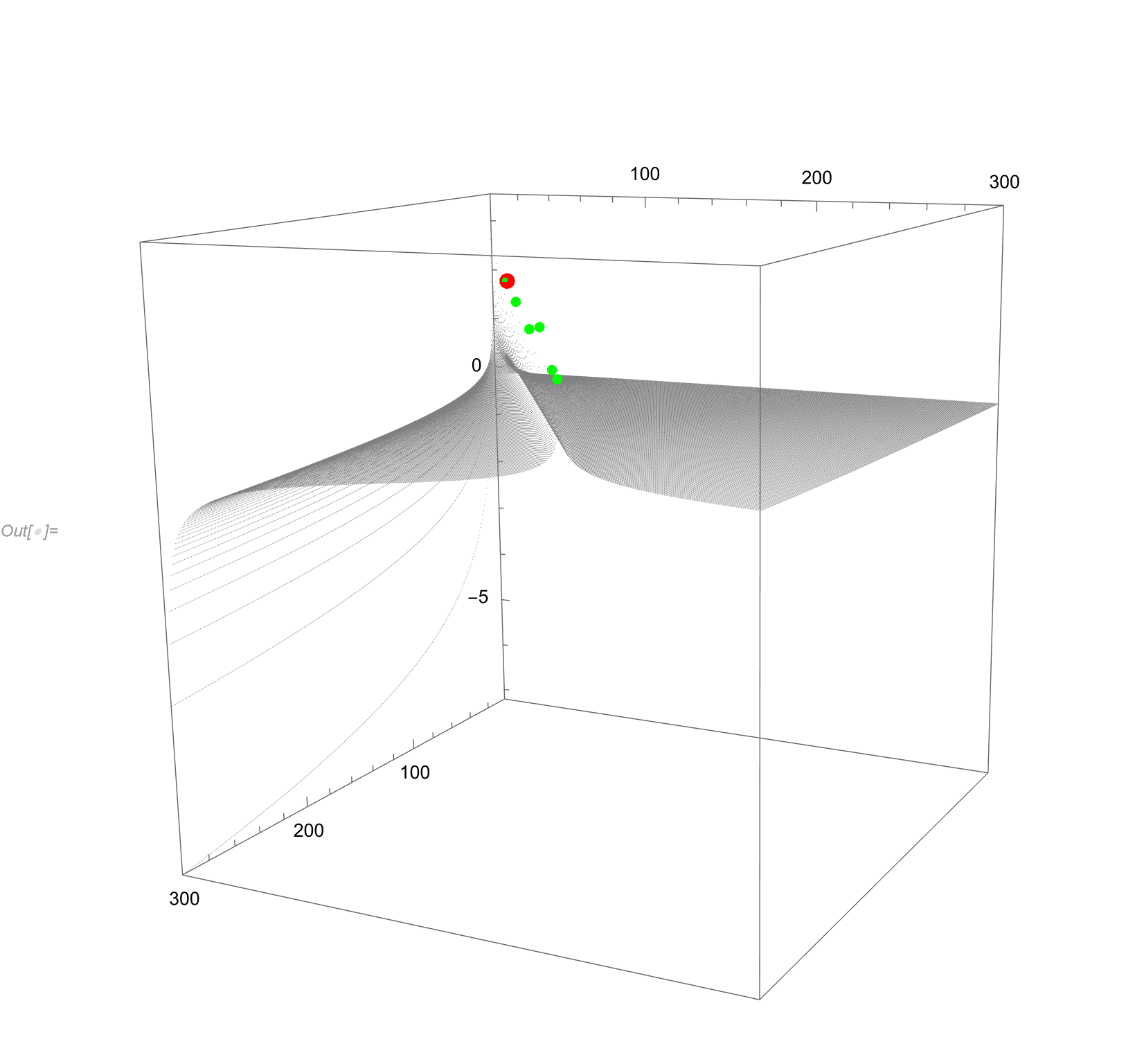
3D plot of candidate points satisfying constraints

This is just an extended comment. Many times constructing a figure helps one focus on a solution. Below the gray dots are the values of Log[1/y, Abs[Sqrt[2] - x/y]], the green dots are the values where Abs[Sqrt[2] - x/y] <= 0.0001, and the red dot is where the maximum for x>=1&&x<=300&&y>=2&&y<=300 occurs.

ϵ = 1/10000;
t = Flatten[Table[{x, y, Log[1/y, Abs[Sqrt[2] - x/y]]}, {x, 1, 300}, {y, 2,  300}], 1];

t0 = Select[t, Abs[Sqrt[2] - #[[1]]/#[[2]]] < ϵ &];
(* {{99, 70, -(Log[99/70 - Sqrt[2]]/Log[70])}, 
    {140, 99, -(Log[-(140/99) + Sqrt[2]]/Log[99])}, 
    {198, 140, -(Log[99/70 - Sqrt[2]]/Log[140])},
    {239, 169, -(Log[-(239/169) + Sqrt[2]]/Log[169])},
    {280, 198, -(Log[-(140/99) + Sqrt[2]]/Log[198])},
    {297, 210, -(Log[99/70 - Sqrt[2]]/Log[210])}} *)

tmax = Select[t0, #[[3]] == Max[t0[[All, 3]]] &]
(* {99, 70, -(Log[99/70 - Sqrt[2]]/Log[70])} *)

ListPointPlot3D[{t, t0, tmax}, SphericalRegion -> True, BoxRatios -> {1, 1, 1},
  RotationAction -> "Clip", ImageSize -> Large, PlotRange -> All, 
  PlotStyle -> {{Gray, PointSize[0.001]}, {Green, PointSize[0.01]}, {Red, PointSize[0.015]}}]

3D plot of candidate points satisfying constraints

Source Link
JimB
  • 42.9k
  • 3
  • 51
  • 108

This is just an extended comment. Many times constructing a figure helps one focus on a solution. Below the gray dots are the values of Log[1/y, Abs[Sqrt[2] - x/y]], the green dots are the values where Abs[Sqrt[2] - x/y] <= 0.0001, and the red dot is where the maximum occurs.

ϵ = 1/10000;
t = Flatten[Table[{x, y, Log[1/y, Abs[Sqrt[2] - x/y]]}, {x, 1, 300}, {y, 2,  300}], 1];

t0 = Select[t, Abs[Sqrt[2] - #[[1]]/#[[2]]] < ϵ &];
(* {{99, 70, -(Log[99/70 - Sqrt[2]]/Log[70])}, 
    {140, 99, -(Log[-(140/99) + Sqrt[2]]/Log[99])}, 
    {198, 140, -(Log[99/70 - Sqrt[2]]/Log[140])},
    {239, 169, -(Log[-(239/169) + Sqrt[2]]/Log[169])},
    {280, 198, -(Log[-(140/99) + Sqrt[2]]/Log[198])},
    {297, 210, -(Log[99/70 - Sqrt[2]]/Log[210])}} *)

tmax = Select[t0, #[[3]] == Max[t0[[All, 3]]] &]
(* {99, 70, -(Log[99/70 - Sqrt[2]]/Log[70])} *)

ListPointPlot3D[{t, t0, tmax}, SphericalRegion -> True, BoxRatios -> {1, 1, 1},
  RotationAction -> "Clip", ImageSize -> Large, PlotRange -> All, 
  PlotStyle -> {{Gray, PointSize[0.001]}, {Green, PointSize[0.01]}, {Red, PointSize[0.015]}}]

3D plot of candidate points satisfying constraints