Fixed typo in code.
Source Link
bbgodfrey
  • 62.1k
  • 18
  • 92
  • 160

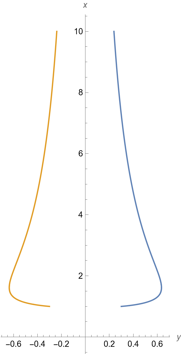
I do not believe that your second DSolve gives the inverse of y. In any case, it is easy to plot the inverse. With Ulrich Neumann's answer as a starting plot, use

ParametricPlot[{{(y[x] /. sol)[[2]] /. {y1 -> 3/10, a -> 13/10, b -> 7/10}, x},
                {(y[x] /. sol)[[1]] /. {y1 -> 3/10, a -> 13/10, b -> 7/10}, x}}, 
                {x, 1, 10}, AspectRatio -> 2, AxesLabel -> {y, x}]

enter image description here

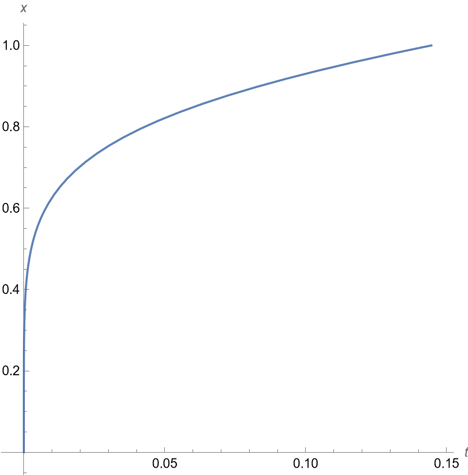
However, if you really do wish to plot the result of the second DSolve, designate it as soli and extract an equation for t as a function of x.

soli[[1, 1, 2, 1]] == soli[[1, 1, 2, 0, 1]][x]
Sqrt[10] # & /@ % /. {a -> 4, b -> 0, C[1] -> 1, C[2] -> 0}

(* t == (Sqrt[5/2] Sqrt[1 + x^10] Hypergeometric2F1[1/2, 3/5, 8/5, 
       -x^10])/(3 Sqrt[10/x^12 + 10/x^2]) *)

(I have chosen the constants for convenience. Other values also work.) Then, use ParametricPlot as before.

ParametricPlot[{%%[[2]], x}, {x, 0, 1}, AspectRatio -> 1, AxesLabel -> {t, x}]

enter image description here

There are, of course, other ways to plot inverses of functions. The method shown seems simplest to me

I do not believe that your second DSolve gives the inverse of y. In any case, it is easy to plot the inverse. With Ulrich Neumann's answer as a starting plot, use

ParametricPlot[{{(y[x] /. sol)[[2]] /. {y1 -> 3/10, a -> 13/10, b -> 7/10}, x},
                {(y[x] /. sol)[[1]] /. {y1 -> 3/10, a -> 13/10, b -> 7/10}, x}}, 
                {x, 1, 10}, AspectRatio -> 2, AxesLabel -> {y, x}]

enter image description here

However, if you really do wish to plot the result of the second DSolve, designate it as soli and extract an equation for t as a function of x.

soli[[1, 1, 2, 1]] == soli[[1, 1, 2, 0, 1]][x]
Sqrt[10] # & /@ % /. {a -> 4, b -> 0, C[1] -> 1, C[2] -> 0}

(* t == (Sqrt[5/2] Sqrt[1 + x^10] Hypergeometric2F1[1/2, 3/5, 8/5, 
       -x^10])/(3 Sqrt[10/x^12 + 10/x^2]) *)

(I have chosen the constants for convenience. Other values also work.) Then, use ParametricPlot as before.

ParametricPlot[{%, x}, {x, 0, 1}, AspectRatio -> 1, AxesLabel -> {t, x}]

enter image description here

There are, of course, other ways to plot inverses of functions. The method shown seems simplest to me
I do not believe that your second DSolve gives the inverse of y. In any case, it is easy to plot the inverse. With Ulrich Neumann's answer as a starting plot, use

ParametricPlot[{{(y[x] /. sol)[[2]] /. {y1 -> 3/10, a -> 13/10, b -> 7/10}, x},
                {(y[x] /. sol)[[1]] /. {y1 -> 3/10, a -> 13/10, b -> 7/10}, x}}, 
                {x, 1, 10}, AspectRatio -> 2, AxesLabel -> {y, x}]

enter image description here

However, if you really do wish to plot the result of the second DSolve, designate it as soli and extract an equation for t as a function of x.

soli[[1, 1, 2, 1]] == soli[[1, 1, 2, 0, 1]][x]
Sqrt[10] # & /@ % /. {a -> 4, b -> 0, C[1] -> 1, C[2] -> 0}

(* t == (Sqrt[5/2] Sqrt[1 + x^10] Hypergeometric2F1[1/2, 3/5, 8/5, 
       -x^10])/(3 Sqrt[10/x^12 + 10/x^2]) *)

(I have chosen the constants for convenience. Other values also work.) Then, use ParametricPlot as before.

ParametricPlot[{%[[2]], x}, {x, 0, 1}, AspectRatio -> 1, AxesLabel -> {t, x}]

enter image description here

There are, of course, other ways to plot inverses of functions. The method shown seems simplest to me

Added sentence
Source Link
bbgodfrey
  • 62.1k
  • 18
  • 92
  • 160

I do not believe that your second DSolve gives the inverse of y. In any case, it is easy to plot the inverse. Using With Ulrich Neumann's answer as a starting plot, use

ParametricPlot[{{(y[x] /. sol)[[2]] /. {y1 -> 3/10, a -> 13/10, b -> 7/10}, x},
                {(y[x] /. sol)[[1]] /. {y1 -> 3/10, a -> 13/10, b -> 7/10}, x}}, 
                {x, 1, 10}, AspectRatio -> 2, AxesLabel -> {y, x}]

enter image description here

However, if you really do wish to plot the result of the second DSolve, designate it as soli and extract an equation for t as a function of x.

soli[[1, 1, 2, 1]] == soli[[1, 1, 2, 0, 1]][x]
Sqrt[10] # & /@ % /. {a -> 4, b -> 0, C[1] -> 1, C[2] -> 0}

(* t == (Sqrt[5/2] Sqrt[1 + x^10] Hypergeometric2F1[1/2, 3/5, 8/5, 
       -x^10])/(3 Sqrt[10/x^12 + 10/x^2]) *)

(I have chosen the constants for convenience. Other values also work.) Then, use ParametricPlot as before.

ParametricPlot[{%, x}, {x, 0, 1}, AspectRatio -> 1, AxesLabel -> {t, x}]

enter image description here

There are, of course, other ways to plot inverses of functions. The method shown seems simplest to me

I do not believe that your second DSolve gives the inverse of y. In any case, it is easy to plot the inverse. Using Ulrich Neumann's answer as a starting plot, use

ParametricPlot[{{(y[x] /. sol)[[2]] /. {y1 -> 3/10, a -> 13/10, b -> 7/10}, x},
                {(y[x] /. sol)[[1]] /. {y1 -> 3/10, a -> 13/10, b -> 7/10}, x}}, 
                {x, 1, 10}, AspectRatio -> 2, AxesLabel -> {y, x}]

enter image description here

However, if you really do wish to plot the result of the second DSolve, designate it as soli and extract an equation for t as a function of x.

soli[[1, 1, 2, 1]] == soli[[1, 1, 2, 0, 1]][x]
Sqrt[10] # & /@ % /. {a -> 4, b -> 0, C[1] -> 1, C[2] -> 0}

(* t == (Sqrt[5/2] Sqrt[1 + x^10] Hypergeometric2F1[1/2, 3/5, 8/5, 
       -x^10])/(3 Sqrt[10/x^12 + 10/x^2]) *)

(I have chosen the constants for convenience. Other values also work.) Then, use ParametricPlot as before.

ParametricPlot[{%, x}, {x, 0, 1}, AspectRatio -> 1, AxesLabel -> {t, x}]

enter image description here

I do not believe that your second DSolve gives the inverse of y. In any case, it is easy to plot the inverse. With Ulrich Neumann's answer as a starting plot, use

ParametricPlot[{{(y[x] /. sol)[[2]] /. {y1 -> 3/10, a -> 13/10, b -> 7/10}, x},
                {(y[x] /. sol)[[1]] /. {y1 -> 3/10, a -> 13/10, b -> 7/10}, x}}, 
                {x, 1, 10}, AspectRatio -> 2, AxesLabel -> {y, x}]

enter image description here

However, if you really do wish to plot the result of the second DSolve, designate it as soli and extract an equation for t as a function of x.

soli[[1, 1, 2, 1]] == soli[[1, 1, 2, 0, 1]][x]
Sqrt[10] # & /@ % /. {a -> 4, b -> 0, C[1] -> 1, C[2] -> 0}

(* t == (Sqrt[5/2] Sqrt[1 + x^10] Hypergeometric2F1[1/2, 3/5, 8/5, 
       -x^10])/(3 Sqrt[10/x^12 + 10/x^2]) *)

(I have chosen the constants for convenience. Other values also work.) Then, use ParametricPlot as before.

ParametricPlot[{%, x}, {x, 0, 1}, AspectRatio -> 1, AxesLabel -> {t, x}]

enter image description here

There are, of course, other ways to plot inverses of functions. The method shown seems simplest to me

Source Link
bbgodfrey
  • 62.1k
  • 18
  • 92
  • 160

I do not believe that your second DSolve gives the inverse of y. In any case, it is easy to plot the inverse. Using Ulrich Neumann's answer as a starting plot, use

ParametricPlot[{{(y[x] /. sol)[[2]] /. {y1 -> 3/10, a -> 13/10, b -> 7/10}, x},
                {(y[x] /. sol)[[1]] /. {y1 -> 3/10, a -> 13/10, b -> 7/10}, x}}, 
                {x, 1, 10}, AspectRatio -> 2, AxesLabel -> {y, x}]

enter image description here

However, if you really do wish to plot the result of the second DSolve, designate it as soli and extract an equation for t as a function of x.

soli[[1, 1, 2, 1]] == soli[[1, 1, 2, 0, 1]][x]
Sqrt[10] # & /@ % /. {a -> 4, b -> 0, C[1] -> 1, C[2] -> 0}

(* t == (Sqrt[5/2] Sqrt[1 + x^10] Hypergeometric2F1[1/2, 3/5, 8/5, 
       -x^10])/(3 Sqrt[10/x^12 + 10/x^2]) *)

(I have chosen the constants for convenience. Other values also work.) Then, use ParametricPlot as before.

ParametricPlot[{%, x}, {x, 0, 1}, AspectRatio -> 1, AxesLabel -> {t, x}]

enter image description here