added 568 characters in body
Source Link
LouisB
  • 12.8k
  • 1
  • 22
  • 34

To summarize, the two results are different because the second method uses equations that are linearly dependent for some functions. By themselves, they do not contain enough information to determine a unique solution.

Long answer: Take a look at Eqs 12-14 in the link that you cited and imagine all of the $a_i=1$, as in your example. All of those equations would then be the same, not independent. Now look at Eq 15 and imagine all of the $a_i=1$. The first $M$ rows would be identical, so the determinant would be zero.

But, it's even worse than that. You don't have to imagine all of the $a_i=1$. It is only $a_{L-M+1} \dots a_{L+M}$ that appear in Eqs 12-14. So in your example, you could change $a_0$ and $a_1$ and get the same non-answer. And, of course, it's the $a_i$'s being equal to one another, not necessarily equal to 1, that makes the determinant zero.

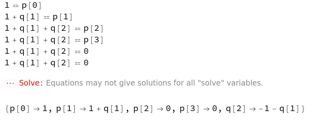
The following code generates Eqs 7-11 and Eqs 12-14 for the subject polynomial function and attempts to solve the system of equations.

l = 3; m = 2;
rules = {q[0] -> 1, a[_?(# < 0 &)] -> 0, q[_?(# > m &)] -> 0};
eqns7$11 = Table[Sum[a[j] q[irow - j], {j, 0, irow}] == p[irow],
    {irow, 0, l}] /. rules;
eqns12$14 = Table[Sum[a[l - j + irow] q[j], {j, 0, m}] == 0,
    {irow, m}] /. rules;

(eqns = Join[eqns7$11, eqns12$14] /. a[_] -> 1) // Column
soln = First@Solve[eqns]

enter image description here

The Solve solution allows either $q_1$ or $q_2$ to be a free parameter. Setting $q_2=0$ gives $q_1=-1$, in agreement with the PadeApproximant result.

Let's try different choices of q[1] and see what we get for the approximant

    ϕ = Sum[p[k] x^k, {k, 0, l}]/Sum[q[k] x^k, {k, 0, m}]
    ϕ //. Flatten@{q[0] -> 1, soln, q[1] -> -1}
    ϕ //. Flatten@{q[0] -> 1, soln, q[1] -> 0} // Simplify
    ϕ //. Flatten@{q[0] -> 1, soln, q[1] -> 1} // Simplify

(* 
(p[0] + x p[1] + x^2 p[2] + x^3 p[3])/(q[0] + x q[1] + x^2 q[2])
1/(1 - x)
1/(1 - x)
1/(1 - x)  *)

Simplify was used in the above to cancel common polynomial factors in numerator and the denominator.

To summarize, the two results are different because the second method uses equations that are linearly dependent for some functions. By themselves, they do not contain enough information to determine a unique solution.

Long answer: Take a look at Eqs 12-14 in the link that you cited and imagine all of the $a_i=1$, as in your example. All of those equations would then be the same, not independent. Now look at Eq 15 and imagine all of the $a_i=1$. The first $M$ rows would be identical, so the determinant would be zero.

But, it's even worse than that. You don't have to imagine all of the $a_i=1$. It is only $a_{L-M+1} \dots a_{L+M}$ that appear in Eqs 12-14. So in your example, you could change $a_0$ and $a_1$ and get the same non-answer. And, of course, it's the $a_i$'s being equal to one another, not necessarily equal to 1, that makes the determinant zero.

The following code generates Eqs 7-11 and Eqs 12-14 for the subject polynomial function and attempts to solve the system of equations.

l = 3; m = 2;
rules = {q[0] -> 1, a[_?(# < 0 &)] -> 0, q[_?(# > m &)] -> 0};
eqns7$11 = Table[Sum[a[j] q[irow - j], {j, 0, irow}] == p[irow],
    {irow, 0, l}] /. rules;
eqns12$14 = Table[Sum[a[l - j + irow] q[j], {j, 0, m}] == 0,
    {irow, m}] /. rules;

(eqns = Join[eqns7$11, eqns12$14] /. a[_] -> 1) // Column
soln = First@Solve[eqns]

enter image description here

The Solve solution allows either $q_1$ or $q_2$ to be a free parameter. Setting $q_2=0$ gives $q_1=-1$, in agreement with the PadeApproximant result.

Let's try different choices of q[1] and see what we get for the approximant

    ϕ = Sum[p[k] x^k, {k, 0, l}]/Sum[q[k] x^k, {k, 0, m}]
    ϕ //. Flatten@{q[0] -> 1, soln, q[1] -> -1}
    ϕ //. Flatten@{q[0] -> 1, soln, q[1] -> 0} // Simplify
    ϕ //. Flatten@{q[0] -> 1, soln, q[1] -> 1} // Simplify

(* 
(p[0] + x p[1] + x^2 p[2] + x^3 p[3])/(q[0] + x q[1] + x^2 q[2])
1/(1 - x)
1/(1 - x)
1/(1 - x)  *)

Simplify was used in the above to cancel common polynomial factors in numerator and the denominator.

Source Link
LouisB
  • 12.8k
  • 1
  • 22
  • 34

To summarize, the two results are different because the second method uses equations that are linearly dependent for some functions. By themselves, they do not contain enough information to determine a unique solution.

Long answer: Take a look at Eqs 12-14 in the link that you cited and imagine all of the $a_i=1$, as in your example. All of those equations would then be the same, not independent. Now look at Eq 15 and imagine all of the $a_i=1$. The first $M$ rows would be identical, so the determinant would be zero.

But, it's even worse than that. You don't have to imagine all of the $a_i=1$. It is only $a_{L-M+1} \dots a_{L+M}$ that appear in Eqs 12-14. So in your example, you could change $a_0$ and $a_1$ and get the same non-answer. And, of course, it's the $a_i$'s being equal to one another, not necessarily equal to 1, that makes the determinant zero.

The following code generates Eqs 7-11 and Eqs 12-14 for the subject polynomial function and attempts to solve the system of equations.

l = 3; m = 2;
rules = {q[0] -> 1, a[_?(# < 0 &)] -> 0, q[_?(# > m &)] -> 0};
eqns7$11 = Table[Sum[a[j] q[irow - j], {j, 0, irow}] == p[irow],
    {irow, 0, l}] /. rules;
eqns12$14 = Table[Sum[a[l - j + irow] q[j], {j, 0, m}] == 0,
    {irow, m}] /. rules;

(eqns = Join[eqns7$11, eqns12$14] /. a[_] -> 1) // Column
soln = First@Solve[eqns]

enter image description here

The Solve solution allows either $q_1$ or $q_2$ to be a free parameter. Setting $q_2=0$ gives $q_1=-1$, in agreement with the PadeApproximant result.