added more
Source Link
Hugh
  • 16.8k
  • 3
  • 32
  • 85

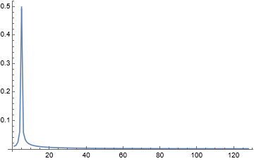
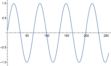
Here is an example of how to use FourierParameters for interpolating a spectrum. First we generate some data, take the ordinary Fourier transform and plot.

data = Table[Sin[\[Pi] k/33], {k, 256}] // N;
ListLinePlot[data]
ft = Fourier[data, FourierParameters -> {-1, -1}];
ListLinePlot[Abs@ft[[1 ;; 128]], PlotRange -> All]
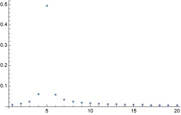
ListPlot[Abs@ft[[1 ;; 20]], PlotRange -> All]

enter image description here

enter image description here

enter image description here

The last, expanded view of the spectrum shows that there are rather few points defining the peak.

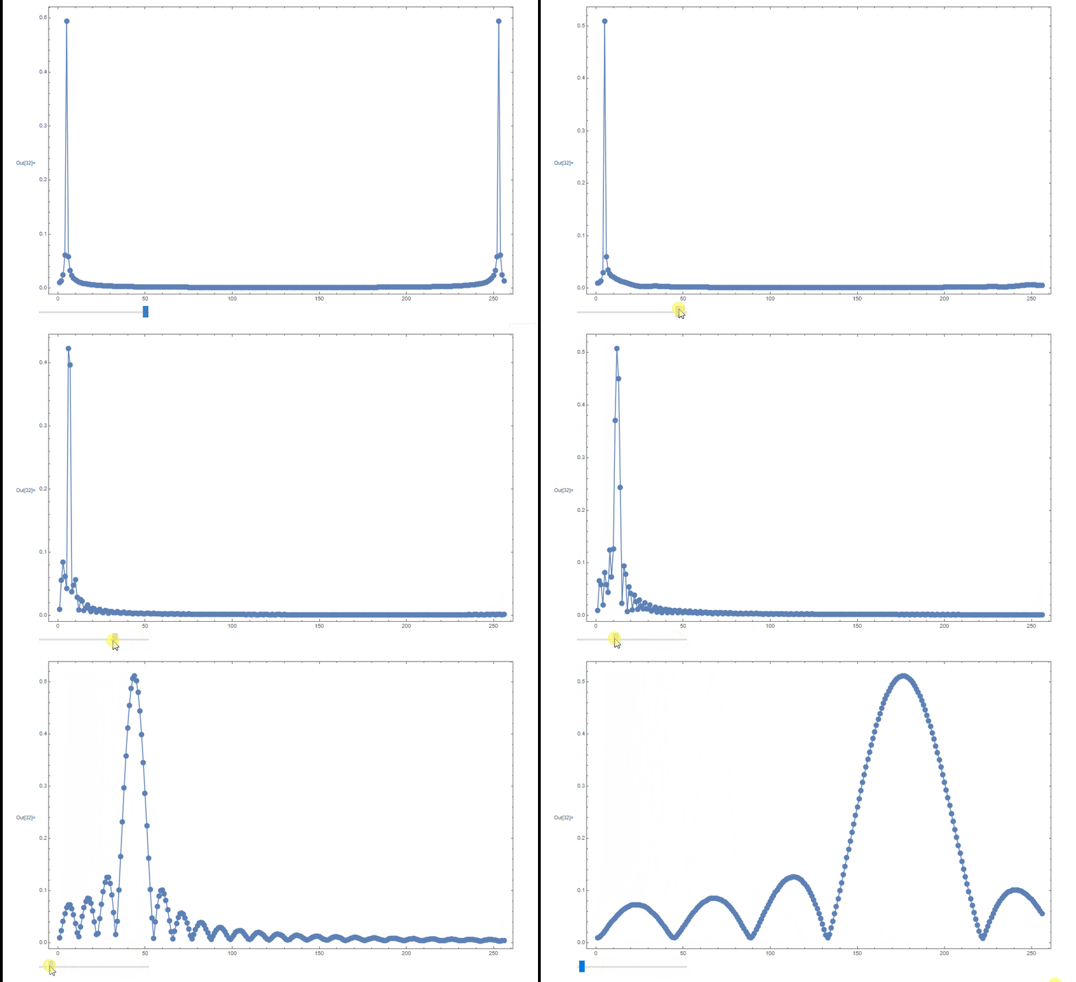
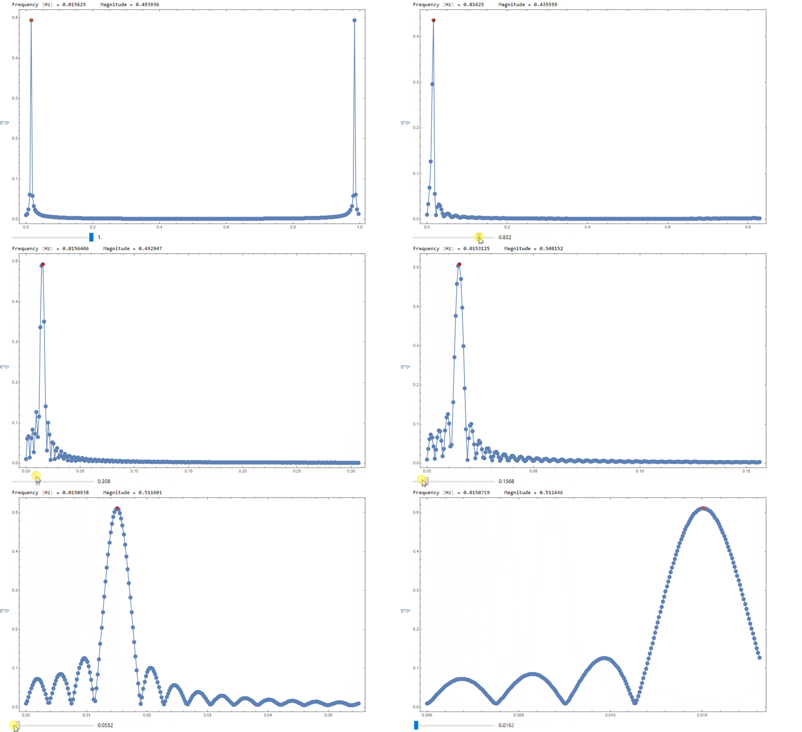
The following Dynamic enables the interpolation to be seen when FourierParameters are altered. The actual frequency and the magnitude of the Fourier peak should be

 (*   {0.0151515, 0.511146}   *)

DynamicModule[{b = 1, pos, a = 0, ft, freqs},
 ft = Fourier[dataAbs@Fourier[data, FourierParameters -> {-1, b}];
 pos = Position[ft, Max[ft]][[1, 1]];
 freqs = Table[(n - 1)/Length[data], {n, Length[data]}];
 Column[{
   Dynamic@Dynamic[
    ListLinePlot[Abs@ft[[1Row[{"Frequency ;;(Hz) 256]]= ", a[[1]], "     Magnitude = ", a[[2]] }]],
   Dynamic@ListLinePlot[Transpose[{freqs, ft}], PlotRange -> All,
     Epilog -> {Red, PointSize[0.01], 
       Point[a = Transpose[{freqs, ft}][[pos]]]},
     ImageSize -> 12 72, Frame -> True, Mesh -> All],
   Slider[
    Dynamic[bSlider[Dynamic[b, {b = #; 
       ft = Fourier[dataAbs@Fourier[data, FourierParameters -> {-1, b}]];
       freqs = Table[b (n - 1)/Length[data], {n, Length[data]}];
       pos = Position[ft, Max[ft]][[1, 1]]
       } &], {0, 1}], Appearance -> "Labeled"]
   }]
 ]

enter image description hereenter image description here

As you can see we can get many more points into the peak and have thus interpolated the spectrum. Thus we can more accurately work out the frequency.

Give me some more time and I will try and add a frequency scale to the plots.

Hope that helps.

Here is an example of how to use FourierParameters for interpolating a spectrum. First we generate some data, take the ordinary Fourier transform and plot.

data = Table[Sin[\[Pi] k/33], {k, 256}] // N;
ListLinePlot[data]
ft = Fourier[data, FourierParameters -> {-1, -1}];
ListLinePlot[Abs@ft[[1 ;; 128]], PlotRange -> All]
ListPlot[Abs@ft[[1 ;; 20]], PlotRange -> All]

enter image description here

enter image description here

enter image description here

The last, expanded view of the spectrum shows that there are rather few points defining the peak.

The following Dynamic enables the interpolation to be seen when FourierParameters are altered.

    DynamicModule[{b = 1},
 ft = Fourier[data, FourierParameters -> {-1, b}];
 Column[{
   Dynamic@
    ListLinePlot[Abs@ft[[1 ;; 256]], PlotRange -> All, 
     ImageSize -> 12 72, Frame -> True, Mesh -> All],
   Slider[
    Dynamic[b, {b = #; 
       ft = Fourier[data, FourierParameters -> {-1, b}]} &], {0, 1}]
   }]
 ]

enter image description here

As you can see we can get many more points into the peak and have thus interpolated the spectrum. Thus we can more accurately work out the frequency.

Give me some more time and I will try and add a frequency scale to the plots.

Hope that helps.
Here is an example of how to use FourierParameters for interpolating a spectrum. First we generate some data, take the ordinary Fourier transform and plot.

data = Table[Sin[\[Pi] k/33], {k, 256}] // N;
ListLinePlot[data]
ft = Fourier[data, FourierParameters -> {-1, -1}];
ListLinePlot[Abs@ft[[1 ;; 128]], PlotRange -> All]
ListPlot[Abs@ft[[1 ;; 20]], PlotRange -> All]

enter image description here

enter image description here

enter image description here

The last, expanded view of the spectrum shows that there are rather few points defining the peak.

The following Dynamic enables the interpolation to be seen when FourierParameters are altered. The actual frequency and the magnitude of the Fourier peak should be

 (*   {0.0151515, 0.511146}   *)

DynamicModule[{b = 1, pos, a = 0, ft, freqs},
 ft = Abs@Fourier[data, FourierParameters -> {-1, b}];
 pos = Position[ft, Max[ft]][[1, 1]];
 freqs = Table[(n - 1)/Length[data], {n, Length[data]}];
 Column[{
   Dynamic[
    Row[{"Frequency (Hz) = ", a[[1]], "     Magnitude = ", a[[2]] }]],
   Dynamic@ListLinePlot[Transpose[{freqs, ft}], PlotRange -> All,
     Epilog -> {Red, PointSize[0.01], 
       Point[a = Transpose[{freqs, ft}][[pos]]]},
     ImageSize -> 12 72, Frame -> True, Mesh -> All],
   Slider[Dynamic[b, {b = #;
       ft = Abs@Fourier[data, FourierParameters -> {-1, b}];
       freqs = Table[b (n - 1)/Length[data], {n, Length[data]}];
       pos = Position[ft, Max[ft]][[1, 1]]
       } &], {0, 1}, Appearance -> "Labeled"]
   }]
 ]

enter image description here

As you can see we can get many more points into the peak and have thus interpolated the spectrum. Thus we can more accurately work out the frequency.

Hope that helps.

Source Link
Hugh
  • 16.8k
  • 3
  • 32
  • 85

Here is an example of how to use FourierParameters for interpolating a spectrum. First we generate some data, take the ordinary Fourier transform and plot.

data = Table[Sin[\[Pi] k/33], {k, 256}] // N;
ListLinePlot[data]
ft = Fourier[data, FourierParameters -> {-1, -1}];
ListLinePlot[Abs@ft[[1 ;; 128]], PlotRange -> All]
ListPlot[Abs@ft[[1 ;; 20]], PlotRange -> All]

enter image description here

enter image description here

enter image description here

The last, expanded view of the spectrum shows that there are rather few points defining the peak.

The following Dynamic enables the interpolation to be seen when FourierParameters are altered.

    DynamicModule[{b = 1},
 ft = Fourier[data, FourierParameters -> {-1, b}];
 Column[{
   Dynamic@
    ListLinePlot[Abs@ft[[1 ;; 256]], PlotRange -> All, 
     ImageSize -> 12 72, Frame -> True, Mesh -> All],
   Slider[
    Dynamic[b, {b = #; 
       ft = Fourier[data, FourierParameters -> {-1, b}]} &], {0, 1}]
   }]
 ]

enter image description here

As you can see we can get many more points into the peak and have thus interpolated the spectrum. Thus we can more accurately work out the frequency.

Give me some more time and I will try and add a frequency scale to the plots.

Hope that helps.