added 1930 characters in body
Source Link
kglr
  • 400.5k
  • 18
  • 488
  • 929

Update: AnAs an alternative and more flexible approach: Post, we can post-process ContourPlot output to inject contour labels:.

ClearAll[addLabels]
addLabels[colors_, labels_: Automatic, threshold_: 1/3]3][g_Graphics] := 
  Module[{diag = ArcLength @ Line[TransposeArcLength@Line[Transpose @ PlotRange @ #]g],
   
   assoc = AssociationThread[colors, 
     labels /. Automatic ->  
       MapIndexed[Framed[Style["(" <> ToString @ #2[[1]]ToString@#2[[1]] <> ")", #, 12], 
        FrameStyle -> None, Background -> White, 
        FrameMargins -> Small] &, colors]]}, 
    ReplaceAll[{d_Directive, l__Line} :> 
     {d, l, 
     Module[{BSF = BSplineFunction[First@#], 
        pos = If[ArcLength[#] < diag threshold, {.5}, 
         If[Norm[Subtract @@ #[[1, {1, -1}]]] <= 
           diag threshold, {.3, .8}, {0, 1}]]}, 
       Text[assoc@FirstCase[d, _?ColorQ], #] & /@ (BSF /@ pos)] & /@ {l}}]@#]&] @*@ NormalNormal[g]]

addLabels[colors_, labels_: Automatic, threshold_: 1/3][Legended[g_, legend_]] := 
 Legended[addLabels[colors, labels, threshold] @ g, legend]

The first argument, colors, is a list of colors with the same length as functionlist in ContourPlot[functionlist,...].

The (optional) second argument, labels, is a list of labels with the same length (if this argument is Automatic or not provided, the labels are taken to be numbers from 1 to length of colors).

The third argument, threshold, is also optional and it is used to control the number of labels and label positions on a contour curve. If a contour curve is too short (in comparison to the length of the diagonal of the plotting area) then a single label is placed in the middle of the curve. If the start and end points of the curve not too close two labels are placed at the two ends of the curve. If they are too close (as in a closed curve) two labels are placed so that they are not too close to each other.

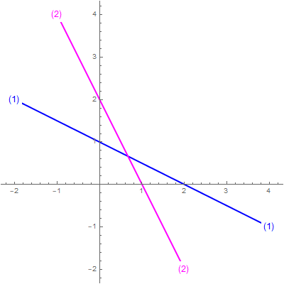
We can use addLabels in two ways: (1) as the the setting for the option DisplayFunction by adding the option DisplayFunction -> addLabels[colors, labels, threshold] to ContourPlot, or (2) by wrapping ContourPlot[...] with it, i.e., using addLabels[colors, labels, threshold] @ ContourPlot[...].

{g1, g2, b} = {x + 2 y, 2 x + y, {2, 2}};

funcs = {g1 - b[[1]], g2 - b[[2]]};

colors = {Blue, Magenta};

plotoptions = {Frame -> False, Axes -> True, ContourShading -> None, 
   ImageSize -> 400, PlotRangePadding -> Scaled[.05]};

ContourPlot[funcs, {x, -2, 4}, {y, -2, 4}, Frame 
 ->Evaluate False@ options, 
   AxesContourStyle -> TrueThread[Directive[colors, 
 Thick]],  
 ContourStyleDisplayFunction -> Thread[Directive[colors,addLabels[colors]]

enter image description here

addLabels[colors] Thick]]@ ContourPlot[funcs, 
 {x, -2, 4}, ImageSize{y, ->2, 4004}, 
   PlotRangePadding  Evaluate @ options, ContourStyle -> Scaled[.05]];

addLabels[colors]@plotThread[Directive[colors, Thick]]]

enter image description here

 same picture
funcs = {g1 - b[[1]], g2 - b[[2]], Cos[x - 1] + Cos[y - 1] - 1/3, 
   Sin[ x - 1] + x y Cos[y + 1] - 1/4}; 

colors = {Blue, Magenta, Red, Green};

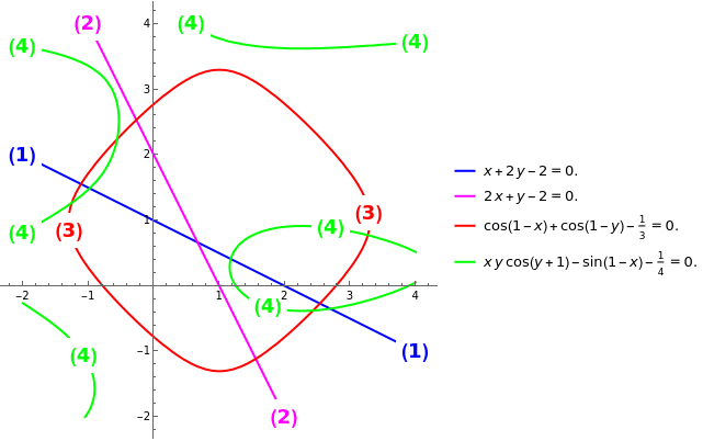
addLabels[colors]@plot gives we get

enter image description hereenter image description here

labels = MapIndexed[Framed[Style["(" <> ToString@#2[[1]] <> ")", #, Bold, 18], 
     FrameStyle -> None, Background -> White] &, colors];

addLabels[colorsContourPlot[funcs, labels]{x, -2, 4}, {y, -2, 4},
 Evaluate @ plotoptions,
 ContourStyle -> Thread[Directive[colors, Thick]], 
 DisplayFunction -> addLabels[colors, labels]]

enter image description hereenter image description here

Add the option PlotLegends->"Expressions" to get

enter image description here

Update: An alternative approach: Post-process ContourPlot output to inject contour labels:

ClearAll[addLabels]
addLabels[colors_, labels_: Automatic, threshold_: 1/3] := 
 Module[{diag = ArcLength @ Line[Transpose @ PlotRange @ #],
     assoc = AssociationThread[colors, labels /. Automatic ->  
       MapIndexed[Framed[Style["(" <> ToString @ #2[[1]] <> ")", #, 12], 
        FrameStyle -> None, Background -> White, 
        FrameMargins -> Small] &, colors]]}, 
    ReplaceAll[{d_Directive, l__Line} :> 
     {d, l, Module[{BSF = BSplineFunction[First@#], 
       pos = If[ArcLength[#] < diag threshold, {.5}, 
        If[Norm[Subtract @@ #[[1, {1, -1}]]] <= diag threshold, {.3, .8}, {0, 1}]]}, 
      Text[assoc@FirstCase[d, _?ColorQ], #] & /@ (BSF /@ pos)] & /@ {l}}]@#]& @* Normal
{g1, g2, b} = {x + 2 y, 2 x + y, {2, 2}};

funcs = {g1 - b[[1]], g2 - b[[2]]};

colors = {Blue, Magenta};

plot = ContourPlot[funcs, {x, -2, 4}, {y, -2, 4}, Frame -> False, 
   Axes -> True, 
   ContourStyle -> Thread[Directive[colors, Thick]], 
    ImageSize -> 400,
   PlotRangePadding -> Scaled[.05]];

addLabels[colors]@plot

enter image description here

funcs = {g1 - b[[1]], g2 - b[[2]], Cos[x - 1] + Cos[y - 1] - 1/3, 
   Sin[ x - 1] + x y Cos[y + 1] - 1/4};
colors = {Blue, Magenta, Red, Green};

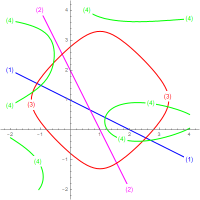
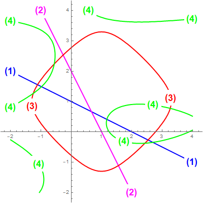
addLabels[colors]@plot gives

enter image description here

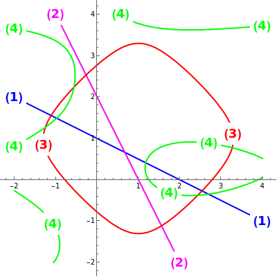
labels = MapIndexed[Framed[Style["(" <> ToString@#2[[1]] <> ")", #, Bold, 18], 
     FrameStyle -> None, Background -> White] &, colors];

addLabels[colors, labels] @ plot

enter image description here

Update: As an alternative and more flexible approach, we can post-process ContourPlot output to inject contour labels.

ClearAll[addLabels]
addLabels[colors_, labels_: Automatic, threshold_: 1/3][g_Graphics] :=
  Module[{diag = ArcLength@Line[Transpose @ PlotRange @ g],  
   assoc = AssociationThread[colors, 
     labels /. Automatic -> 
       MapIndexed[Framed[Style["(" <> ToString@#2[[1]] <> ")", #, 12], 
        FrameStyle -> None, Background -> White, FrameMargins -> Small] &, colors]]}, 
  ReplaceAll[{d_Directive, l__Line} :> {d, l, 
     Module[{BSF = BSplineFunction[First@#], 
        pos = If[ArcLength[#] < diag threshold, {.5}, 
         If[Norm[Subtract @@ #[[1, {1, -1}]]] <= 
           diag threshold, {.3, .8}, {0, 1}]]}, 
       Text[assoc@FirstCase[d, _?ColorQ], #] & /@ (BSF /@ pos)] & /@ {l}}] @ Normal[g]]

addLabels[colors_, labels_: Automatic, threshold_: 1/3][Legended[g_, legend_]] := 
 Legended[addLabels[colors, labels, threshold] @ g, legend]

The first argument, colors, is a list of colors with the same length as functionlist in ContourPlot[functionlist,...].

The (optional) second argument, labels, is a list of labels with the same length (if this argument is Automatic or not provided, the labels are taken to be numbers from 1 to length of colors).

The third argument, threshold, is also optional and it is used to control the number of labels and label positions on a contour curve. If a contour curve is too short (in comparison to the length of the diagonal of the plotting area) then a single label is placed in the middle of the curve. If the start and end points of the curve not too close two labels are placed at the two ends of the curve. If they are too close (as in a closed curve) two labels are placed so that they are not too close to each other.

We can use addLabels in two ways: (1) as the the setting for the option DisplayFunction by adding the option DisplayFunction -> addLabels[colors, labels, threshold] to ContourPlot, or (2) by wrapping ContourPlot[...] with it, i.e., using addLabels[colors, labels, threshold] @ ContourPlot[...].

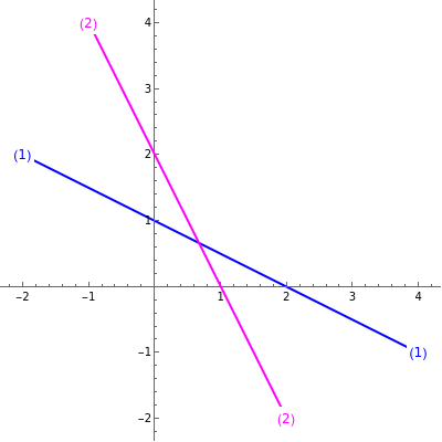
{g1, g2, b} = {x + 2 y, 2 x + y, {2, 2}};

funcs = {g1 - b[[1]], g2 - b[[2]]};

colors = {Blue, Magenta};

options = {Frame -> False, Axes -> True, ContourShading -> None, 
   ImageSize -> 400, PlotRangePadding -> Scaled[.05]};

ContourPlot[funcs, {x, -2, 4}, {y, -2, 4},  
 Evaluate @ options, 
 ContourStyle -> Thread[Directive[colors, Thick]],  
 DisplayFunction -> addLabels[colors]]

enter image description here

addLabels[colors] @ ContourPlot[funcs, {x, -2, 4}, {y, -2, 4}, 
     Evaluate @ options, ContourStyle -> Thread[Directive[colors, Thick]]]
 same picture
funcs = {g1 - b[[1]], g2 - b[[2]], Cos[x - 1] + Cos[y - 1] - 1/3, 
   Sin[ x - 1] + x y Cos[y + 1] - 1/4}; 

colors = {Blue, Magenta, Red, Green};

we get

enter image description here

labels = MapIndexed[Framed[Style["(" <> ToString@#2[[1]] <> ")", #, Bold, 18], 
     FrameStyle -> None, Background -> White] &, colors];

ContourPlot[funcs, {x, -2, 4}, {y, -2, 4},
 Evaluate @ options,
 ContourStyle -> Thread[Directive[colors, Thick]], 
 DisplayFunction -> addLabels[colors, labels]]

enter image description here

Add the option PlotLegends->"Expressions" to get
enter image description here

deleted 20 characters in body
Source Link
kglr
  • 400.5k
  • 18
  • 488
  • 929
labels = MapIndexed[Framed[Style["(" <> ToString@#2[[1]] <> ")", #, Bold, 18], 
     FrameStyle -> None, Background -> White] &, coloresRest];colors];

addLabels[colors, labels] @ plot
{g1, g2, b} = {x + 2 y, 2 x + y, {2, 2}};

coloresRestcolors = {Blue, Magenta};

labels = MapIndexed[Framed[Style["(" <> ToString@#2[[1]] <> ")", #, 18], 
     FrameStyle -> None, Background -> White] &, coloresRest];colors];

Show[MapThread[
      ContourPlot[#, {x, -2, 4}, {y, -2, 4}, 
         Frame -> False, 
         Axes -> True,
         ContourShading -> None, 
         Contours -> {0}, 
         ContourStyle -> Directive[#2, Thick], 
         ContourLabels -> Function[{x, y, z}, Text[#3, {x, y}]], 
         ImageSize -> 400] &, 
      {{g1 - b[[1]], g2 - b[[2]]}, coloresRestcolors, labels}]] 
labels = MapIndexed[Framed[Style["(" <> ToString@#2[[1]] <> ")", #, Bold, 18], 
     FrameStyle -> None, Background -> White] &, coloresRest];

addLabels[colors, labels] @ plot
{g1, g2, b} = {x + 2 y, 2 x + y, {2, 2}};

coloresRest = {Blue, Magenta};

labels = MapIndexed[Framed[Style["(" <> ToString@#2[[1]] <> ")", #, 18], 
     FrameStyle -> None, Background -> White] &, coloresRest];

Show[MapThread[
      ContourPlot[#, {x, -2, 4}, {y, -2, 4}, 
         Frame -> False, 
         Axes -> True,
         ContourShading -> None, 
         Contours -> {0}, 
         ContourStyle -> Directive[#2, Thick], 
         ContourLabels -> Function[{x, y, z}, Text[#3, {x, y}]], 
         ImageSize -> 400] &, 
      {{g1 - b[[1]], g2 - b[[2]]}, coloresRest, labels}]] 
labels = MapIndexed[Framed[Style["(" <> ToString@#2[[1]] <> ")", #, Bold, 18], 
     FrameStyle -> None, Background -> White] &, colors];

addLabels[colors, labels] @ plot
{g1, g2, b} = {x + 2 y, 2 x + y, {2, 2}};

colors = {Blue, Magenta};

labels = MapIndexed[Framed[Style["(" <> ToString@#2[[1]] <> ")", #, 18], 
     FrameStyle -> None, Background -> White] &, colors];

Show[MapThread[
      ContourPlot[#, {x, -2, 4}, {y, -2, 4}, 
         Frame -> False, 
         Axes -> True,
         ContourShading -> None, 
         Contours -> {0}, 
         ContourStyle -> Directive[#2, Thick], 
         ContourLabels -> Function[{x, y, z}, Text[#3, {x, y}]], 
         ImageSize -> 400] &, 
      {{g1 - b[[1]], g2 - b[[2]]}, colors, labels}]] 
added 1979 characters in body
Source Link
kglr
  • 400.5k
  • 18
  • 488
  • 929
{g1, g2, b} = {x + 2 y, 2 x + y, {2, 2}};

funcs = {g1 - b[[1]], g2 - b[[2]]}; 

colors = {Blue, Magenta};

plot = ContourPlot[funcs, {x, -2, 4}, {y, -2, 4}, Frame -> False, 
   Axes -> True, 
   ContourStyle -> Thread[Directive[colors, Thick]], 
   ImageSize -> 400,
   PlotRangePadding -> Scaled[.05]];

addLabels[colors]@plot

1addLabels[colors]@plot`addLabels[colors]@plot gives

funcs = {g1 - b[[1]], g2 - b[[2]]};
colors = {Blue, Magenta};

plot = ContourPlot[funcs, {x, -2, 4}, {y, -2, 4}, Frame -> False, 
   Axes -> True, 
   ContourStyle -> Thread[Directive[colors, Thick]], 
   ImageSize -> 400,
   PlotRangePadding -> Scaled[.05]];

addLabels[colors]@plot

1addLabels[colors]@plot` gives

{g1, g2, b} = {x + 2 y, 2 x + y, {2, 2}};

funcs = {g1 - b[[1]], g2 - b[[2]]}; 

colors = {Blue, Magenta};

plot = ContourPlot[funcs, {x, -2, 4}, {y, -2, 4}, Frame -> False, 
   Axes -> True, 
   ContourStyle -> Thread[Directive[colors, Thick]], 
   ImageSize -> 400,
   PlotRangePadding -> Scaled[.05]];

addLabels[colors]@plot

addLabels[colors]@plot gives

added 1979 characters in body
Source Link
kglr
  • 400.5k
  • 18
  • 488
  • 929
Loading
added 44 characters in body
Source Link
kglr
  • 400.5k
  • 18
  • 488
  • 929
Loading
Source Link
kglr
  • 400.5k
  • 18
  • 488
  • 929
Loading