added 9 characters in body
Source Link

You can use FourierCoefficient to pre-calculate the Fourier coefficients to arbitrary degree and then use the result very effectively.

There may be some issues with zero-th degree, therefore I excluded this using Piecewise. Here's the main code block:

f[x_] := Piecewise[{
    {-x^3 - 2 x, -2 < x < 0},
    {-1 + x, 0 <= x <= 2}},
    0
];
    Module[{x, fp},
    (* Set parameters so that the integration runs
       from -2 to 2 *)
    fp = {0, -Pi/2};
    fc = Piecewise[{
        {FourierCoefficient[f[x], x, 0, FourierParameters -> fp], # == 0},
        {ComplexExpand@FourierCoefficient[f[x], x, #, FourierParameters -> fp], True}
    }] &;
    fc = Evaluate /@ fc;
];

The output (fc) of this is something very unpleasant to look at; however, there's nothing Fourier-related left there, all the hard math has been done already, and only a bunch of elementary functions remain. fc is now a function of one argument that gives you the n$n$-th Fourier coefficient of f in no time.

(* Calculate the first 2001 Fourier coefficients *)
AbsoluteTiming[Table[fc[n], {n, -1000, 1000}]] // First
0.777059 seconds

To convert this back to the function, you have to do the partial sum with your hands, for example here are the second, fourth and eighietheightieth partial sums:

myPartialSums = Table[
    (* 1/2 andThe Pi/2 compensatecompensates for the custom FourierParameters, see
       documentation of FourierSeries/FourierParameters
       under "more info" *)
    1/2 Re[Sum[fc[k] Exp[PiExp[-Pi/2 I k t], {k, -n, n}]],
    {n, {2, 4, 80}}
];
A very large output has been generated,
but we're luckily not interested in it
anyway but would rather plot it

Plot[
    {f[t]}~Join~myPartialSums ~Join~ myPartialSums,
    {t, -10, 10},
    PlotRange -> All, 
    Evaluated -> True, 
    PlotStyle -> {Thick, Automatic, Automatic, Automatic}
]

enter image description hereplot of Fourier series partial sums

You can use FourierCoefficient to pre-calculate the Fourier coefficients to arbitrary degree and then use the result very effectively.

There may be some issues with zero-th degree, therefore I excluded this using Piecewise. Here's the main code block:

f[x_] := Piecewise[{
    {-x^3 - 2 x, -2 < x < 0},
    {-1 + x, 0 <= x <= 2}},
    0
];
    Module[{x, fp},
    (* Set parameters so that the integration runs
       from -2 to 2 *)
    fp = {0, Pi/2};
    fc = Piecewise[{
        {FourierCoefficient[f[x], x, 0, FourierParameters -> fp], # == 0},
        {ComplexExpand@FourierCoefficient[f[x], x, #, FourierParameters -> fp], True}
    }] &;
    fc = Evaluate /@ fc;
];

The output (fc) of this is something very unpleasant to look at; however, there's nothing Fourier-related left there, all the hard math has been done already, and only a bunch of elementary functions remain. fc is now a function of one argument that gives you the n-th Fourier coefficient of f in no time.

(* Calculate the first 2001 Fourier coefficients *)
AbsoluteTiming[Table[fc[n], {n, -1000, 1000}]] // First
0.777059 seconds

To convert this back to the function, you have to do the partial sum with your hands, for example here are the second, fourth and eighieth partial sums:

myPartialSums = Table[
    (* 1/2 and Pi/2 compensate the custom FourierParameters, see
       documentation of FourierSeries/FourierParameters
       under "more info" *)
    1/2 Re[Sum[fc[k] Exp[Pi/2 I k t], {k, -n, n}]],
    {n, {2, 4, 80}}
];
A very large output has been generated,
but we're luckily not interested in it
anyway but would rather plot it

Plot[
    {f[t]}~Join~myPartialSums,
    {t, -10, 10},
    PlotRange -> All, 
    Evaluated -> True, 
    PlotStyle -> {Thick, Automatic, Automatic, Automatic}
]
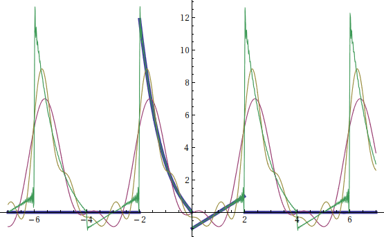
enter image description here

You can use FourierCoefficient to pre-calculate the Fourier coefficients to arbitrary degree and then use the result very effectively.

There may be some issues with zero-th degree, therefore I excluded this using Piecewise. Here's the main code block:

f[x_] := Piecewise[{
    {-x^3 - 2 x, -2 < x < 0},
    {-1 + x, 0 <= x <= 2}},
    0
];
    Module[{x, fp},
    (* Set parameters so that the integration runs
       from -2 to 2 *)
    fp = {0, -Pi/2};
    fc = Piecewise[{
        {FourierCoefficient[f[x], x, 0, FourierParameters -> fp], # == 0},
        {ComplexExpand@FourierCoefficient[f[x], x, #, FourierParameters -> fp], True}
    }] &;
    fc = Evaluate /@ fc;
];

The output (fc) of this is something very unpleasant to look at; however, there's nothing Fourier-related left there, all the hard math has been done already, and only a bunch of elementary functions remain. fc is now a function of one argument that gives you the $n$-th Fourier coefficient of f in no time.

(* Calculate the first 2001 Fourier coefficients *)
AbsoluteTiming[Table[fc[n], {n, -1000, 1000}]] // First
0.777059 seconds

To convert this back to the function, you have to do the partial sum with your hands, for example here are the second, fourth and eightieth partial sums:

myPartialSums = Table[
    (* The Pi/2 compensates for the custom FourierParameters, see
       documentation of FourierSeries/FourierParameters
       under "more info" *)
    Re[Sum[fc[k] Exp[-Pi/2 I k t], {k, -n, n}]],
    {n, {2, 4, 80}}
];
A very large output has been generated,
but we're luckily not interested in it
anyway but would rather plot it

Plot[
    {f[t]} ~Join~ myPartialSums,
    {t, -10, 10},
    PlotRange -> All, 
    Evaluated -> True, 
    PlotStyle -> {Thick, Automatic, Automatic, Automatic}
]

plot of Fourier series partial sums

added 33 characters in body
Source Link
David
  • 15k
  • 6
  • 51
  • 82
f[x_] := Piecewise[{
    {-x^3 - 2 x, -2 < x < 0},
    {-1 + x, 0 <= x <= 2}},
    0
];
    Module[{x, fp},
    fc =(* Piecewise[{
Set parameters so that the integration runs
  {FourierCoefficient[f[x], x, 0], # == 0},
from -2 to 2 *)
    {ComplexExpand@FourierCoefficient[f[x],fp x,= #]{0, TruePi/2};
    }]fc &;= Piecewise[{
    (* Evaluate the contents of{FourierCoefficient[f[x], thex, above0, definedFourierParameters pure-> fp], # == 0},
       function to{ComplexExpand@FourierCoefficient[f[x], dox, the#, actualFourierParameters pre-calculation> *)fp], True}
    }] &;
    fc = Evaluate /@ fc;
  ];

The output (fc) of this is something very unpleasant along the lines of

enter image description here

(This would be more compact, but harder to manipulate using Re/Im, if I hadn't used ComplexExpand in the module above.)

Howeverlook at; however, you can clearly see that there's nothing Fourier-related left there, all the hard math has been done already, and only a bunch of elementary functions remain. fc is now a function of one argument that gives you the n-th Fourier coefficient of f in no time.

To convert this back to the function, you have to do the partial sum with your hands, for example here are the second, fourth and eightheighieth partial sums:

myPartialSums = Table[
    (* 1/2 and Pi/2 compensate the custom FourierParameters, see
       documentation of FourierSeries/FourierParameters
       under "more info" *)
    1/2 Re[Sum[fc[k] Exp[IExp[Pi/2 I k t], {k, -n, n}]],
    {n, {2, 4, 880}}
]];

enter image description hereenter image description here

f[x_] := Piecewise[{
    {-x^3 - 2 x, -2 < x < 0},
    {-1 + x, 0 <= x <= 2}},
    0
];
Module[{x},
    fc = Piecewise[{
        {FourierCoefficient[f[x], x, 0], # == 0},
        {ComplexExpand@FourierCoefficient[f[x], x, #], True}
    }] &;
    (* Evaluate the contents of the above defined pure
       function to do the actual pre-calculation *)
    fc = Evaluate /@ fc;
  ];

The output (fc) of this is something unpleasant along the lines of

enter image description here

(This would be more compact, but harder to manipulate using Re/Im, if I hadn't used ComplexExpand in the module above.)

However, you can clearly see that there's nothing Fourier-related left there, all the hard math has been done already. fc is now a function of one argument that gives you the n-th Fourier coefficient of f in no time.

To convert this back to the function, you have to do the partial sum with your hands, for example here are the second, fourth and eighth partial sums:

myPartialSums = Table[
    Re[Sum[fc[k] Exp[I k t], {k, -n, n}]],
    {n, {2, 4, 8}}
]

enter image description here

f[x_] := Piecewise[{
    {-x^3 - 2 x, -2 < x < 0},
    {-1 + x, 0 <= x <= 2}},
    0
];
    Module[{x, fp},
    (* Set parameters so that the integration runs
       from -2 to 2 *)
    fp = {0, Pi/2};
    fc = Piecewise[{
        {FourierCoefficient[f[x], x, 0, FourierParameters -> fp], # == 0},
        {ComplexExpand@FourierCoefficient[f[x], x, #, FourierParameters -> fp], True}
    }] &;
    fc = Evaluate /@ fc;
];

The output (fc) of this is something very unpleasant to look at; however, there's nothing Fourier-related left there, all the hard math has been done already, and only a bunch of elementary functions remain. fc is now a function of one argument that gives you the n-th Fourier coefficient of f in no time.

To convert this back to the function, you have to do the partial sum with your hands, for example here are the second, fourth and eighieth partial sums:

myPartialSums = Table[
    (* 1/2 and Pi/2 compensate the custom FourierParameters, see
       documentation of FourierSeries/FourierParameters
       under "more info" *)
    1/2 Re[Sum[fc[k] Exp[Pi/2 I k t], {k, -n, n}]],
    {n, {2, 4, 80}}
];

enter image description here

added 9 characters in body
Source Link
David
  • 15k
  • 6
  • 51
  • 82

You can use FourierCoefficient to pre-calculate the Fourier coefficients to arbitrary degree and then use the result very effectively.

There may be some issues with zero-th degree, therefore I excluded this using Piecewise. Here's the main code block:

f[x_] := Piecewise[{
    {-x^3 - 2 x, -2 < x < 0},
    {-1 + x, 0 <= x <= 2}},
    0
];
Module[{x},
    fc = Piecewise[{
        {FourierCoefficient[f[x], x, 0], # == 0},
        {ComplexExpand@FourierCoefficient[f[x], x, #], True}
    }] &;
    (* Evaluate the contents of the above defined pure
       function to do the actual pre-calculation *)
    fc = Evaluate /@ fc;
  ];

The output (fc) of this is something unpleasant along the lines of

enter image description here

(This would be more compact, but harder to manipulate using Re/Im, if I hadn't used ComplexExpand in the module above.)

However, you can clearly see that there's nothing Fourier-related left there, all the hard math has been done already. fc is now a function of one argument that gives you the n-th Fourier coefficient of f in no time.

(* Calculate the first 2012001 Fourier coefficients *)
AbsoluteTiming[Table[fc[n], {n, 100-1000, 1000}]] // First
0.018575777059 seconds

To convert this back to the function, you have to do the partial sum with your hands, for example here are the second, fourth and eighth partial sums:

myPartialSums = Table[
    Re[Sum[fc[k] Exp[I k t], {k, -n, n}]],
    {n, {2, 4, 8}}
]
A very large output has been generated,
but we're luckily not interested in it
anyway but would rather plot it

Plot[
    {f[t]}~Join~myPartialSums,
    {t, -10, 10},
    PlotRange -> All, 
    Evaluated -> True, 
    PlotStyle -> {Thick, Automatic, Automatic, Automatic}
]
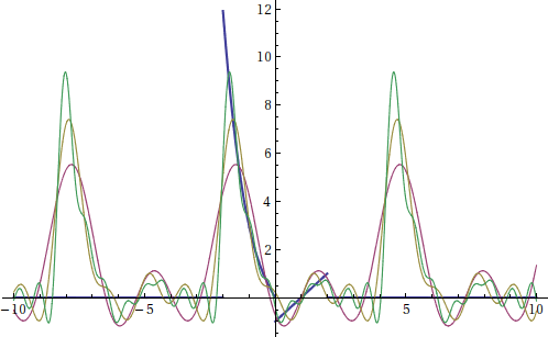
enter image description here

You can use FourierCoefficient to pre-calculate the Fourier coefficients to arbitrary degree and then use the result very effectively.

There may be some issues with zero-th degree, therefore I excluded this using Piecewise. Here's the main code block:

f[x_] := Piecewise[{
    {-x^3 - 2 x, -2 < x < 0},
    {-1 + x, 0 <= x <= 2}},
    0
];
Module[{x},
    fc = Piecewise[{
        {FourierCoefficient[f[x], x, 0], # == 0},
        {ComplexExpand@FourierCoefficient[f[x], x, #], True}
    }] &;
    (* Evaluate the contents of the above defined pure
       function to do the actual pre-calculation *)
    fc = Evaluate /@ fc;
  ];

The output (fc) of this is something unpleasant along the lines of

enter image description here

(This would be more compact, but harder to manipulate using Re/Im, if I hadn't used ComplexExpand in the module above.)

However, you can clearly see that there's nothing Fourier-related left there, all the hard math has been done already. fc is now a function of one argument that gives you the n-th Fourier coefficient of f in no time.

(* Calculate the first 201 Fourier coefficients *)
AbsoluteTiming[Table[fc[n], {n, 100}]] // First
0.018575 seconds

To convert this back to the function, you have to do the partial sum with your hands, for example here are the second, fourth and eighth partial sums:

myPartialSums = Table[
    Re[Sum[fc[k] Exp[I k t], {k, -n, n}]],
    {n, {2, 4, 8}}
]
A very large output has been generated,
but we're luckily not interested in it
anyway but would rather plot it

Plot[
    {f[t]}~Join~myPartialSums,
    {t, -10, 10},
    PlotRange -> All, 
    Evaluated -> True, 
    PlotStyle -> {Thick, Automatic, Automatic, Automatic}
]

enter image description here

You can use FourierCoefficient to pre-calculate the Fourier coefficients to arbitrary degree and then use the result very effectively.

There may be some issues with zero-th degree, therefore I excluded this using Piecewise. Here's the main code block:

f[x_] := Piecewise[{
    {-x^3 - 2 x, -2 < x < 0},
    {-1 + x, 0 <= x <= 2}},
    0
];
Module[{x},
    fc = Piecewise[{
        {FourierCoefficient[f[x], x, 0], # == 0},
        {ComplexExpand@FourierCoefficient[f[x], x, #], True}
    }] &;
    (* Evaluate the contents of the above defined pure
       function to do the actual pre-calculation *)
    fc = Evaluate /@ fc;
  ];

The output (fc) of this is something unpleasant along the lines of

enter image description here

(This would be more compact, but harder to manipulate using Re/Im, if I hadn't used ComplexExpand in the module above.)

However, you can clearly see that there's nothing Fourier-related left there, all the hard math has been done already. fc is now a function of one argument that gives you the n-th Fourier coefficient of f in no time.

(* Calculate the first 2001 Fourier coefficients *)
AbsoluteTiming[Table[fc[n], {n, -1000, 1000}]] // First
0.777059 seconds

To convert this back to the function, you have to do the partial sum with your hands, for example here are the second, fourth and eighth partial sums:

myPartialSums = Table[
    Re[Sum[fc[k] Exp[I k t], {k, -n, n}]],
    {n, {2, 4, 8}}
]
A very large output has been generated,
but we're luckily not interested in it
anyway but would rather plot it

Plot[
    {f[t]}~Join~myPartialSums,
    {t, -10, 10},
    PlotRange -> All, 
    Evaluated -> True, 
    PlotStyle -> {Thick, Automatic, Automatic, Automatic}
]

enter image description here

Lorem ipsum.
Source Link
David
  • 15k
  • 6
  • 51
  • 82
Loading
Source Link
David
  • 15k
  • 6
  • 51
  • 82
Loading