Bounty Ended with 50 reputation awarded by Math
fixed formatting
Source Link
Chris K
  • 20.4k
  • 3
  • 39
  • 75
β = 0.95; γ = 1; n = 1;
Show[
 PlotEcoPhasePlane[{s, 0.9, 1.1}, {i, -0.1, 0.1}],
 Plot[n - s, {s, 0.9, 1.1}, PlotStyle -> Pink],
 RuleListPlot[{{s -> n, i -> 0}, {s -> (n \[Gamma]γ)/\[Beta]β, i -> n - (n \[Gamma]γ)/\[Beta]β}}, PlotMarkers -> {True, False}]
 ]

enter image description hereenter image description here

\[Beta]β = 4; \[Gamma]γ = 1; n = 1;
Show[
 PlotEcoPhasePlane[{s, 0, 1}, {i, 0, 1}],
 Plot[n - s, {s, 0, n}, PlotStyle -> Pink],
 RuleListPlot[{{s -> n, i -> 0}, {s -> (n \[Gamma]γ)/\[Beta]β, i -> n - (n \[Gamma]γ)/\[Beta]β}}, PlotMarkers -> {False, True}]
]

enter image description hereenter image description here

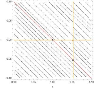
No-disease case (eq[1]eq[[1]] is stable, eq[2]eq[[2]] is a biologically meaningless saddle point):

\[Beta]β = 0.95; \[Gamma]γ = 1; \[Xi]ξ = 1; n = 1;
eq = SolveEcoEq[]
N[EcoEigenvalues[eq[[2]]]]
Show[
 PlotEcoPhasePlane[{s, 0.9, 1.1}, {i, -0.1, 0.1}],
 RuleListPlot[eq, PlotMarkers -> EcoStableQ[eq]]
]
(* {{s -> 1., i -> 0}, {s -> 1.05263, i -> -0.0263158}} *)
(* {-1.02384, 0.0488359} *)

enter image description hereenter image description here

Endemic case 1 (eq[2]eq[[2]] is a stable focus, due to complex eigenvalues):

enter image description hereenter image description here

Endemic case 2 (eq[2]eq[[2]] is a stable node, due to negative real eigenvalues):

enter image description hereenter image description here

β = 0.95; γ = 1; n = 1;
Show[
 PlotEcoPhasePlane[{s, 0.9, 1.1}, {i, -0.1, 0.1}],
 Plot[n - s, {s, 0.9, 1.1}, PlotStyle -> Pink],
 RuleListPlot[{{s -> n, i -> 0}, {s -> (n \[Gamma])/\[Beta], i -> n - (n \[Gamma])/\[Beta]}}, PlotMarkers -> {True, False}]
 ]
enter image description here

\[Beta] = 4; \[Gamma] = 1; n = 1;
Show[
 PlotEcoPhasePlane[{s, 0, 1}, {i, 0, 1}],
 Plot[n - s, {s, 0, n}, PlotStyle -> Pink],
 RuleListPlot[{{s -> n, i -> 0}, {s -> (n \[Gamma])/\[Beta], i -> n - (n \[Gamma])/\[Beta]}}, PlotMarkers -> {False, True}]
]

enter image description here

No-disease case (eq[1] is stable, eq[2] is a biologically meaningless saddle point):

\[Beta] = 0.95; \[Gamma] = 1; \[Xi] = 1; n = 1;
eq = SolveEcoEq[]
N[EcoEigenvalues[eq[[2]]]]
Show[
 PlotEcoPhasePlane[{s, 0.9, 1.1}, {i, -0.1, 0.1}],
 RuleListPlot[eq, PlotMarkers -> EcoStableQ[eq]]
]
(* {{s -> 1., i -> 0}, {s -> 1.05263, i -> -0.0263158}} *)
(* {-1.02384, 0.0488359} *)

enter image description here

Endemic case 1 (eq[2] is a stable focus, due to complex eigenvalues):

enter image description here

Endemic case 2 (eq[2] is a stable node, due to negative real eigenvalues):

enter image description here

β = 0.95; γ = 1; n = 1;
Show[
 PlotEcoPhasePlane[{s, 0.9, 1.1}, {i, -0.1, 0.1}],
 Plot[n - s, {s, 0.9, 1.1}, PlotStyle -> Pink],
 RuleListPlot[{{s -> n, i -> 0}, {s -> (n γ)/β, i -> n - (n γ)/β}}, PlotMarkers -> {True, False}]
 ]

enter image description here

β = 4; γ = 1; n = 1;
Show[
 PlotEcoPhasePlane[{s, 0, 1}, {i, 0, 1}],
 Plot[n - s, {s, 0, n}, PlotStyle -> Pink],
 RuleListPlot[{{s -> n, i -> 0}, {s -> (n γ)/β, i -> n - (n γ)/β}}, PlotMarkers -> {False, True}]
]

enter image description here

No-disease case (eq[[1]] is stable, eq[[2]] is a biologically meaningless saddle point):

β = 0.95; γ = 1; ξ = 1; n = 1;
eq = SolveEcoEq[]
N[EcoEigenvalues[eq[[2]]]]
Show[
 PlotEcoPhasePlane[{s, 0.9, 1.1}, {i, -0.1, 0.1}],
 RuleListPlot[eq, PlotMarkers -> EcoStableQ[eq]]
]
(* {{s -> 1., i -> 0}, {s -> 1.05263, i -> -0.0263158}} *)
(* {-1.02384, 0.0488359} *)

enter image description here

Endemic case 1 (eq[[2]] is a stable focus, due to complex eigenvalues):

enter image description here

Endemic case 2 (eq[[2]] is a stable node, due to negative real eigenvalues):

enter image description here

addressed some questions
Source Link
Chris K
  • 20.4k
  • 3
  • 39
  • 75

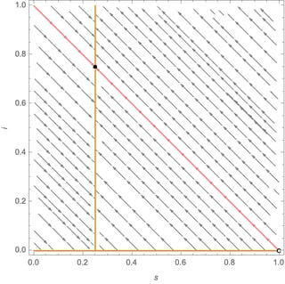
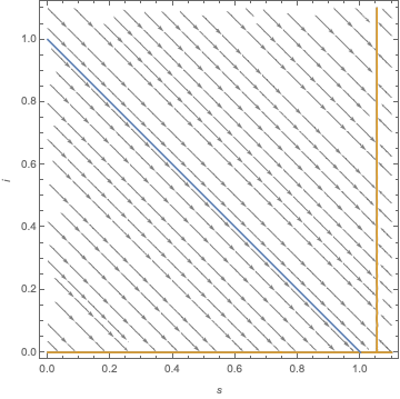
Let's go straight to the phase planes using PlotEcoPhasePlane, manually adding the total population constraint as a pink straight line. The subcriticalno-disease case (disease-free equilibrium eq[[1]] is stable, the other equilibrium eq[[2]] is biologically meaningless since s > n and i < 0):

β = 0.95; γ = 1; n = 1;
Show[
 PlotEcoPhasePlane[{s, 0.9, 1.1}, {i, -0.1, 10.1}],
 Plot[n - s, {s, 0.9, 1.1}, PlotStyle -> Pink], 
 RuleListPlot[{{s -> n, i -> 0}, {s -> (n \[Gamma])/\[Beta], i -> n - (n \[Gamma])/\[Beta]}}, PlotMarkers -> {True, False}]
 ]

enter image description hereenter image description here

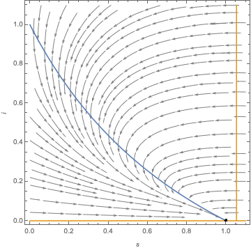
and the supercriticalendemic case (endemic equilibrium eq[[2]] is stable):

β\[Beta] = 4; γ\[Gamma] = 1; n = 1;
Show[
 PlotEcoPhasePlane[{s, 0, 1}, {i, 0, 1}],
 Plot[n - s, {s, 0, n}, PlotStyle -> Pink],
 RuleListPlot[{{s -> n, i -> 0}, {s -> (n \[Gamma])/\[Beta], i -> n - (n \[Gamma])/\[Beta]}}, PlotMarkers -> {False, True}]
]

enter image description hereenter image description here

Again, because of the total-population constraint, this is effectively a one-dimensional system with either two or one feasible (non-negative) equilibria. Note that the two different isoclines ($S$ and $I$) overlap completely because of this and just look gold.

On to the phase planes. The $S$-isocline is blue, to which I will include the equilibria (probably should automate this...)$I$-isocline is gold.

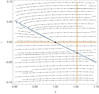
SubcriticalNo-disease case (eq[1] is stable, eq[2] is a biologically meaningless saddle point):

β\[Beta] = 0.95; γ\[Gamma] = 1; ξ\[Xi] = 1; n = 1;
eq = SolveEcoEq[];SolveEcoEq[]
N[EcoEigenvalues[eq[[2]]]]
Show[
 PlotEcoPhasePlane[{s, 0.9, 1.1}, {i, -0.1, 10.1}],
 RuleListPlot[eq, PlotMarkers -> EcoStableQ[eq]]
]
(* {{s -> 1., i -> 0}, {s -> 1.05263, i -> -0.0263158}} *)
(* {-1.02384, 0.0488359} *)
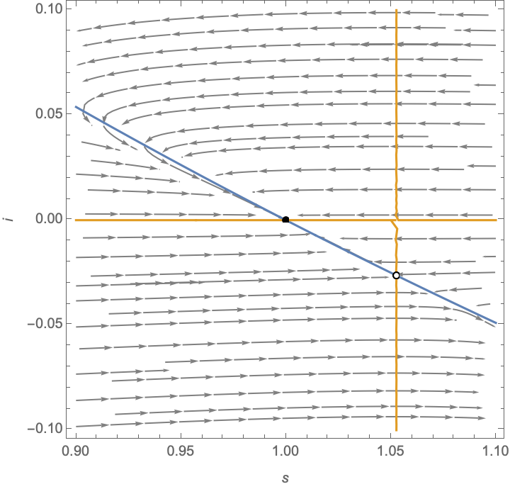
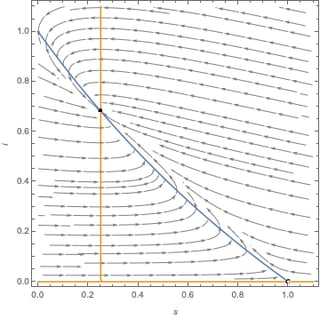
enter image description hereenter image description here

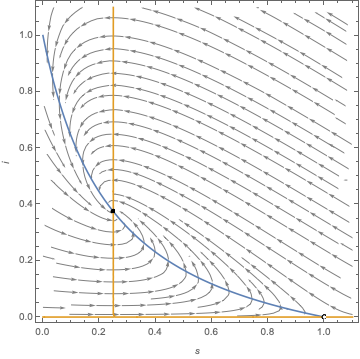
SupercriticalEndemic case 1 (stableeq[2] is a stable focus, due to complex eigenvalues):

β = 4; γ = 1; ξ = 1; n = 1;
eq = SolveEcoEq[];SolveEcoEq[]
N[EcoEigenvalues[eq[[-1]]]]N[EcoEigenvalues[eq[[2]]]]
Show[
 PlotEcoPhasePlane[{s, 0, 1.1}, {i, 0, 1.1}],
 RuleListPlot[eq, PlotMarkers -> EcoStableQ[eq]]
]
(* {{s -> 1, i -> 0}, {s -> 1/4, i -> 3/8}} *)
(* {-1.25 + 1.19896 I, -1.25 - 1.19896 I} *)

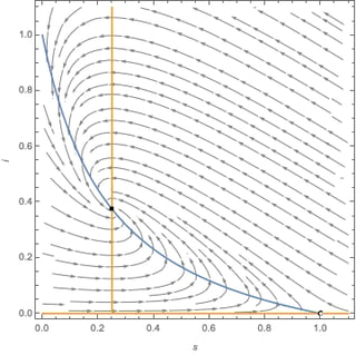
SupercriticalEndemic case 2 (stableeq[2] is a stable node, due to negative real eigenvalues):

β = 4; γ = 1; ξ = 10; n = 1;
eq = SolveEcoEq[];SolveEcoEq[]
N[EcoEigenvalues[eq[[-1]]]]N[EcoEigenvalues[eq[[2]]]]
Show[
 PlotEcoPhasePlane[{s, 0, 1.1}, {i, 0, 1.1}],
 RuleListPlot[eq, PlotMarkers -> EcoStableQ[eq]]
]
(* {{s -> 1, i -> 0}, {s -> 1/4, i -> 15/22}} *)
(* {-9.60337, -3.1239} *)

Let's go straight to the phase planes using PlotEcoPhasePlane, manually adding the total population constraint as a straight line. The subcritical case (disease-free equilibrium eq[[1]] is stable):

β = 0.95; γ = 1; n = 1;
Show[
 PlotEcoPhasePlane[{s, 0, 1.1}, {i, 0, 1.1}],
 Plot[n - s, {s, 0, n}]
]

enter image description here

and the supercritical case (endemic equilibrium eq[[2]] is stable):

β = 4; γ = 1; n = 1;
Show[
 PlotEcoPhasePlane[{s, 0, 1}, {i, 0, 1}],
 Plot[n - s, {s, 0, n}]
]

enter image description here

Again, because of the total-population constraint, this is effectively a one-dimensional system with either two or one feasible (non-negative) equilibria. Note that the two different isoclines ($S$ and $I$) overlap completely because of this.

On to the phase planes, to which I will include the equilibria (probably should automate this...).

Subcritical case:

β = 0.95; γ = 1; ξ = 1; n = 1;
eq = SolveEcoEq[];
Show[
 PlotEcoPhasePlane[{s, 0, 1.1}, {i, 0, 1.1}],
 RuleListPlot[eq, PlotMarkers -> EcoStableQ[eq]]
]

enter image description here

Supercritical case (stable focus, complex eigenvalues):

β = 4; γ = 1; ξ = 1; n = 1;
eq = SolveEcoEq[];
N[EcoEigenvalues[eq[[-1]]]]
Show[
 PlotEcoPhasePlane[{s, 0, 1.1}, {i, 0, 1.1}],
 RuleListPlot[eq, PlotMarkers -> EcoStableQ[eq]]
]
(* {-1.25 + 1.19896 I, -1.25 - 1.19896 I} *)

Supercritical case (stable node, real eigenvalues):

β = 4; γ = 1; ξ = 10; n = 1;
eq = SolveEcoEq[];
N[EcoEigenvalues[eq[[-1]]]]
Show[
 PlotEcoPhasePlane[{s, 0, 1.1}, {i, 0, 1.1}],
 RuleListPlot[eq, PlotMarkers -> EcoStableQ[eq]]
]
(* {-9.60337, -3.1239} *)

Let's go straight to the phase planes using PlotEcoPhasePlane, manually adding the total population constraint as a pink straight line. The no-disease case (disease-free equilibrium eq[[1]] is stable, the other equilibrium eq[[2]] is biologically meaningless since s > n and i < 0):

β = 0.95; γ = 1; n = 1;
Show[
 PlotEcoPhasePlane[{s, 0.9, 1.1}, {i, -0.1, 0.1}],
 Plot[n - s, {s, 0.9, 1.1}, PlotStyle -> Pink], 
 RuleListPlot[{{s -> n, i -> 0}, {s -> (n \[Gamma])/\[Beta], i -> n - (n \[Gamma])/\[Beta]}}, PlotMarkers -> {True, False}]
 ]

enter image description here

and the endemic case (endemic equilibrium eq[[2]] is stable):

\[Beta] = 4; \[Gamma] = 1; n = 1;
Show[
 PlotEcoPhasePlane[{s, 0, 1}, {i, 0, 1}],
 Plot[n - s, {s, 0, n}, PlotStyle -> Pink],
 RuleListPlot[{{s -> n, i -> 0}, {s -> (n \[Gamma])/\[Beta], i -> n - (n \[Gamma])/\[Beta]}}, PlotMarkers -> {False, True}]
]

enter image description here

Again, because of the total-population constraint, this is effectively a one-dimensional system with either two or one feasible (non-negative) equilibria. Note that the two different isoclines ($S$ and $I$) overlap completely because of this and just look gold.

On to the phase planes. The $S$-isocline is blue, the $I$-isocline is gold.

No-disease case (eq[1] is stable, eq[2] is a biologically meaningless saddle point):

\[Beta] = 0.95; \[Gamma] = 1; \[Xi] = 1; n = 1;
eq = SolveEcoEq[]
N[EcoEigenvalues[eq[[2]]]]
Show[
 PlotEcoPhasePlane[{s, 0.9, 1.1}, {i, -0.1, 0.1}],
 RuleListPlot[eq, PlotMarkers -> EcoStableQ[eq]]
]
(* {{s -> 1., i -> 0}, {s -> 1.05263, i -> -0.0263158}} *)
(* {-1.02384, 0.0488359} *)

enter image description here

Endemic case 1 (eq[2] is a stable focus, due to complex eigenvalues):

β = 4; γ = 1; ξ = 1; n = 1;
eq = SolveEcoEq[]
N[EcoEigenvalues[eq[[2]]]]
Show[
 PlotEcoPhasePlane[{s, 0, 1.1}, {i, 0, 1.1}],
 RuleListPlot[eq, PlotMarkers -> EcoStableQ[eq]]
]
(* {{s -> 1, i -> 0}, {s -> 1/4, i -> 3/8}} *)
(* {-1.25 + 1.19896 I, -1.25 - 1.19896 I} *)

Endemic case 2 (eq[2] is a stable node, due to negative real eigenvalues):

β = 4; γ = 1; ξ = 10; n = 1;
eq = SolveEcoEq[]
N[EcoEigenvalues[eq[[2]]]]
Show[
 PlotEcoPhasePlane[{s, 0, 1.1}, {i, 0, 1.1}],
 RuleListPlot[eq, PlotMarkers -> EcoStableQ[eq]]
]
(* {{s -> 1, i -> 0}, {s -> 1/4, i -> 15/22}} *)
(* {-9.60337, -3.1239} *)
added 89 characters in body
Source Link
Chris K
  • 20.4k
  • 3
  • 39
  • 75

Again, because of the total-population constraint, this is effectively a one-dimensional system with either two or one feasible (non-negative) equilibria. Note that the two different isoclines ($S$ and $I$) overlap completely because of this.

r := n - s - i;
SetModel[{
  Pop[pop] -> {
    Component[s] -> {Equation :> -β s i/n + ξ r},
    Component[i] -> {Equation :> β s i/n - γ i}
  },
  Parameters :> {β > 0, γ > 0, ξ > 0, n > 0}
}]

Again, because of the total-population constraint, this is effectively a one-dimensional system with either two or one feasible (non-negative) equilibria.

r := n - s - i;
SetModel[{
  Pop[pop] -> {
    Component[s] -> {Equation :> -β s i/n + ξ r},
    Component[i] -> {Equation :> β s i/n - γ i}
  },
  Parameters :> {β > 0, γ > 0, ξ > 0}
}]

Again, because of the total-population constraint, this is effectively a one-dimensional system with either two or one feasible (non-negative) equilibria. Note that the two different isoclines ($S$ and $I$) overlap completely because of this.

r := n - s - i;
SetModel[{
  Pop[pop] -> {
    Component[s] -> {Equation :> -β s i/n + ξ r},
    Component[i] -> {Equation :> β s i/n - γ i}
  },
  Parameters :> {β > 0, γ > 0, ξ > 0, n > 0}
}]
Source Link
Chris K
  • 20.4k
  • 3
  • 39
  • 75
Loading