Revisions to How to clip several plots in a continuous way

added 1022 characters in body

Source Link

edited Dec 11, 2020 at 21:23

400.5k
18
488
929

An alternative trick is to add a semi-transparent rectangle as Epilog:

With[{a1 = 1, a2 = 2, a = 3, b1 = 1, b2 = 2, b = 3, lag1 = 26, 
  lag = 30, time1 = 40, time2 = 36, time3 = 39}, 
 p1 = Plot[a Sqrt[x] - b Cos[x], {x, 0, time1}, PlotStyle -> Blue];
 p2 = Plot[a1 Sqrt[x] - b1 Cos[x], {x, time1 - lag, time2}, PlotStyle -> Red];
 p3 = Plot[a2 Sqrt[x] - b2 Cos[x], {x, time2 - lag1, time3}, PlotStyle -> Green];
 Show[p1, p2, p3, 
  Epilog -> {Opacity[.8, White], Rectangle[{15, .5}, {40, 40}]}, 
  GridLines -> {{15}, None}, 
  GridLinesStyle -> Directive[Gray, Dashed], PlotRange -> All]]

You can also use the option ColorFunction:

An alternative trick isUpdate: We can use the last approach to add a semi-transparent rectangle as Epiloghave different thresholds in the three plots:

With[DynamicModule[{a1 = 1, a2 = 2, a = 3, b1 = 1, b2 = 2, b = 3, 
  lag1 = 26, 
  lag = 30, time1 = 40, time2 = 36, time3 = 39, 
  thresholds = {15, 20, 25}}, 
 p1 = Plot[a Sqrt[x] - b Cos[x], {x, 0, time1}, PlotStyleMesh -> Blue];{{15}}, 
   ColorFunctionScaling -> False, 
   ColorFunction -> twoToneCF[thresholds[[1]], Blue]];
 p2 = Plot[a1 Sqrt[x] - b1 Cos[x], {x, time1 - lag, time2}, PlotStyle
   ColorFunctionScaling -> Red];False, 
   ColorFunction -> twoToneCF[thresholds[[2]], Red]];
 p3 = Plot[a2 Sqrt[x] - b2 Cos[x], {x, time2 - lag1, time3}, PlotStyle 
 -> Green];
 Show[p1,ColorFunctionScaling p2,-> p3False, 
  Epilog ColorFunction -> {Opacity[.8, White]twoToneCF[thresholds[[3]], Rectangle[{15,Green]];
 0}Show[p1, {40p2, 40}]}p3, 
  GridLines -> {Thread[{15thresholds, {Blue, Red, Green}}], None}, 
  GridLinesStyle -> Directive[Gray, Dashed], PlotRange -> All]]

NoteAn aside: You might want top play with ConditionalExpression and Piecewise to get all three plots using a single Plot.

You can also use the option ColorFunction:

An alternative trick is to add a semi-transparent rectangle as Epilog:

With[{a1 = 1, a2 = 2, a = 3, b1 = 1, b2 = 2, b = 3, lag1 = 26, 
  lag = 30, time1 = 40, time2 = 36, time3 = 39}, 
 p1 = Plot[a Sqrt[x] - b Cos[x], {x, 0, time1}, PlotStyle -> Blue];
 p2 = Plot[a1 Sqrt[x] - b1 Cos[x], {x, time1 - lag, time2}, PlotStyle -> Red];
 p3 = Plot[a2 Sqrt[x] - b2 Cos[x], {x, time2 - lag1, time3}, PlotStyle -> Green];
 Show[p1, p2, p3, 
  Epilog -> {Opacity[.8, White], Rectangle[{15, 0}, {40, 40}]}, 
  GridLines -> {{15}, None}, 
  GridLinesStyle -> Directive[Gray, Dashed], PlotRange -> All]]

Note: You might want top play with ConditionalExpression and Piecewise to get all three plots using a single Plot.

An alternative trick is to add a semi-transparent rectangle as Epilog:

With[{a1 = 1, a2 = 2, a = 3, b1 = 1, b2 = 2, b = 3, lag1 = 26, 
  lag = 30, time1 = 40, time2 = 36, time3 = 39}, 
 p1 = Plot[a Sqrt[x] - b Cos[x], {x, 0, time1}, PlotStyle -> Blue];
 p2 = Plot[a1 Sqrt[x] - b1 Cos[x], {x, time1 - lag, time2}, PlotStyle -> Red];
 p3 = Plot[a2 Sqrt[x] - b2 Cos[x], {x, time2 - lag1, time3}, PlotStyle -> Green];
 Show[p1, p2, p3, 
  Epilog -> {Opacity[.8, White], Rectangle[{15, .5}, {40, 40}]}, 
  GridLines -> {{15}, None}, 
  GridLinesStyle -> Directive[Gray, Dashed], PlotRange -> All]]

You can also use the option ColorFunction:

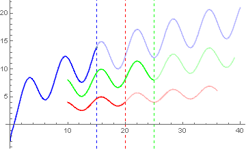
Update: We can use the last approach to have different thresholds in the three plots:

DynamicModule[{a1 = 1, a2 = 2, a = 3, b1 = 1, b2 = 2, b = 3, 
  lag1 = 26, lag = 30, time1 = 40, time2 = 36, time3 = 39, 
  thresholds = {15, 20, 25}}, 
 p1 = Plot[a Sqrt[x] - b Cos[x], {x, 0, time1}, Mesh -> {{15}}, 
   ColorFunctionScaling -> False, 
   ColorFunction -> twoToneCF[thresholds[[1]], Blue]];
 p2 = Plot[a1 Sqrt[x] - b1 Cos[x], {x, time1 - lag, time2}, 
   ColorFunctionScaling -> False, 
   ColorFunction -> twoToneCF[thresholds[[2]], Red]];
 p3 = Plot[a2 Sqrt[x] - b2 Cos[x], {x, time2 - lag1, time3},  
   ColorFunctionScaling -> False, 
   ColorFunction -> twoToneCF[thresholds[[3]], Green]];
 Show[p1, p2, p3, 
  GridLines -> {Thread[{thresholds, {Blue, Red, Green}}], None}, 
  GridLinesStyle -> Directive[Gray, Dashed], PlotRange -> All]]

An aside: You might want top play with ConditionalExpression and Piecewise to get all three plots using a single Plot.

added 1022 characters in body

Source Link

edited Dec 11, 2020 at 21:17

kglr

400.5k
18
488
929

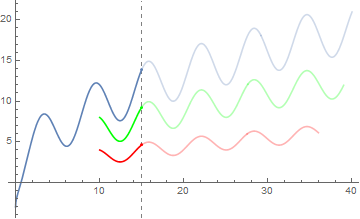
DynamicModule[{a1 = 1, a2 = 2, a = 3, b1 = 1, b2 = 2, b = 3, 
  lag1 = 26, lag = 30, time1 = 40, time2 = 36, time3 = 39}, 
 p1 = Plot[a Sqrt[x] - b Cos[x], {x, 0, time1}, 
   PlotStyle -> Blue, Mesh -> {{15}}, 
   MeshShading -> {Opacity[1], Opacity[0.3]}]; 
 p2 = Plot[a1 Sqrt[x] - b1 Cos[x], {x, time1 - lag, time2}, 
   PlotStyle -> Red, Mesh -> {{15}}, 
   MeshShading -> {Opacity[1], Opacity[0.3]}]; 
 p3 = Plot[a2 Sqrt[x] - b2 Cos[x], {x, time2 - lag1, time3}, 
   PlotStyle -> Green, Mesh -> {{15}}, 
   MeshShading -> {Opacity[1], Opacity[0.3]}]; 
 Show[p1, p2, p3, GridLines -> {{15}, None}, 
  GridLinesStyle -> Directive[Gray, Dashed], PlotRange -> All]]

Note: You might want top play with ConditionalExpression and Piecewise to get all three plots using a singlecan also use the option PlotColorFunction.:

twoToneCF[t_, color_] := If[# <= t, color, Opacity[.3, color]] &;

DynamicModule[{a1 = 1, a2 = 2, a = 3, b1 = 1, b2 = 2, b = 3, 
  lag1 = 26, lag = 30, time1 = 40, time2 = 36, time3 = 39, threshold = 15}, 
 p1 = Plot[a Sqrt[x] - b Cos[x], {x, 0, time1}, Mesh -> {{15}}, 
   ColorFunctionScaling -> False, 
   ColorFunction -> twoToneCF[threshold, Blue]];
 p2 = Plot[a1 Sqrt[x] - b1 Cos[x], {x, time1 - lag, time2}, 
   ColorFunctionScaling -> False, 
   ColorFunction -> twoToneCF[threshold, Red]];
 p3 = Plot[a2 Sqrt[x] - b2 Cos[x], {x, time2 - lag1, time3}, 
   ColorFunctionScaling -> False, 
   ColorFunction -> twoToneCF[threshold, Green]];
 Show[p1, p2, p3, GridLines -> {{threshold}, None}, 
  GridLinesStyle -> Directive[Gray, Dashed], PlotRange -> All]]

With[{a1 = 1, a2 = 2, a = 3, b1 = 1, b2 = 2, b = 3, lag1 = 26, 
  lag = 30, time1 = 40, time2 = 36, time3 = 39}, 
 p1 = Plot[a Sqrt[x] - b Cos[x], {x, 0, time1}];, PlotStyle -> Blue];
 p2 = Plot[a1 Sqrt[x] - b1 Cos[x], {x, time1 - lag, time2}, PlotStyle -> Red];
 p3 = Plot[a2 Sqrt[x] - b2 Cos[x], {x, time2 - lag1, time3}, PlotStyle -> Green];
 Show[p1, p2, p3, 
  Epilog -> {Opacity[.8, White], Rectangle[{15, 0}, {40, 40}]}, 
  GridLines -> {{15}, None}, 
  GridLinesStyle -> Directive[Gray, Dashed], PlotRange -> All]]

Note: You might want top play with ConditionalExpression and Piecewise to get all three plots using a single Plot.

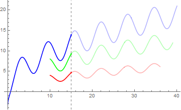
DynamicModule[{a1 = 1, a2 = 2, a = 3, b1 = 1, b2 = 2, b = 3, 
  lag1 = 26, lag = 30, time1 = 40, time2 = 36, time3 = 39}, 
 p1 = Plot[a Sqrt[x] - b Cos[x], {x, 0, time1}, Mesh -> {{15}}, 
   MeshShading -> {Opacity[1], Opacity[0.3]}]; 
 p2 = Plot[a1 Sqrt[x] - b1 Cos[x], {x, time1 - lag, time2}, 
   PlotStyle -> Red, Mesh -> {{15}}, 
   MeshShading -> {Opacity[1], Opacity[0.3]}]; 
 p3 = Plot[a2 Sqrt[x] - b2 Cos[x], {x, time2 - lag1, time3}, 
   PlotStyle -> Green, Mesh -> {{15}}, 
   MeshShading -> {Opacity[1], Opacity[0.3]}]; 
 Show[p1, p2, p3, GridLines -> {{15}, None}, 
  GridLinesStyle -> Directive[Gray, Dashed], PlotRange -> All]]

Note: You might want top play with ConditionalExpression and Piecewise to get all three plots using a single Plot.

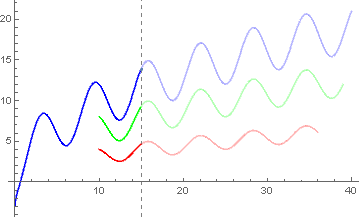
With[{a1 = 1, a2 = 2, a = 3, b1 = 1, b2 = 2, b = 3, lag1 = 26, 
  lag = 30, time1 = 40, time2 = 36, time3 = 39}, 
 p1 = Plot[a Sqrt[x] - b Cos[x], {x, 0, time1}];
 p2 = Plot[a1 Sqrt[x] - b1 Cos[x], {x, time1 - lag, time2}, PlotStyle -> Red];
 p3 = Plot[a2 Sqrt[x] - b2 Cos[x], {x, time2 - lag1, time3}, PlotStyle -> Green];
 Show[p1, p2, p3, 
  Epilog -> {Opacity[.8, White], Rectangle[{15, 0}, {40, 40}]}, 
  GridLines -> {{15}, None}, 
  GridLinesStyle -> Directive[Gray, Dashed], PlotRange -> All]]

DynamicModule[{a1 = 1, a2 = 2, a = 3, b1 = 1, b2 = 2, b = 3, 
  lag1 = 26, lag = 30, time1 = 40, time2 = 36, time3 = 39}, 
 p1 = Plot[a Sqrt[x] - b Cos[x], {x, 0, time1}, 
   PlotStyle -> Blue, Mesh -> {{15}}, 
   MeshShading -> {Opacity[1], Opacity[0.3]}]; 
 p2 = Plot[a1 Sqrt[x] - b1 Cos[x], {x, time1 - lag, time2}, 
   PlotStyle -> Red, Mesh -> {{15}}, 
   MeshShading -> {Opacity[1], Opacity[0.3]}]; 
 p3 = Plot[a2 Sqrt[x] - b2 Cos[x], {x, time2 - lag1, time3}, 
   PlotStyle -> Green, Mesh -> {{15}}, 
   MeshShading -> {Opacity[1], Opacity[0.3]}]; 
 Show[p1, p2, p3, GridLines -> {{15}, None}, 
  GridLinesStyle -> Directive[Gray, Dashed], PlotRange -> All]]

You can also use the option ColorFunction:

twoToneCF[t_, color_] := If[# <= t, color, Opacity[.3, color]] &;

DynamicModule[{a1 = 1, a2 = 2, a = 3, b1 = 1, b2 = 2, b = 3, 
  lag1 = 26, lag = 30, time1 = 40, time2 = 36, time3 = 39, threshold = 15}, 
 p1 = Plot[a Sqrt[x] - b Cos[x], {x, 0, time1}, Mesh -> {{15}}, 
   ColorFunctionScaling -> False, 
   ColorFunction -> twoToneCF[threshold, Blue]];
 p2 = Plot[a1 Sqrt[x] - b1 Cos[x], {x, time1 - lag, time2}, 
   ColorFunctionScaling -> False, 
   ColorFunction -> twoToneCF[threshold, Red]];
 p3 = Plot[a2 Sqrt[x] - b2 Cos[x], {x, time2 - lag1, time3}, 
   ColorFunctionScaling -> False, 
   ColorFunction -> twoToneCF[threshold, Green]];
 Show[p1, p2, p3, GridLines -> {{threshold}, None}, 
  GridLinesStyle -> Directive[Gray, Dashed], PlotRange -> All]]

With[{a1 = 1, a2 = 2, a = 3, b1 = 1, b2 = 2, b = 3, lag1 = 26, 
  lag = 30, time1 = 40, time2 = 36, time3 = 39}, 
 p1 = Plot[a Sqrt[x] - b Cos[x], {x, 0, time1}, PlotStyle -> Blue];
 p2 = Plot[a1 Sqrt[x] - b1 Cos[x], {x, time1 - lag, time2}, PlotStyle -> Red];
 p3 = Plot[a2 Sqrt[x] - b2 Cos[x], {x, time2 - lag1, time3}, PlotStyle -> Green];
 Show[p1, p2, p3, 
  Epilog -> {Opacity[.8, White], Rectangle[{15, 0}, {40, 40}]}, 
  GridLines -> {{15}, None}, 
  GridLinesStyle -> Directive[Gray, Dashed], PlotRange -> All]]

Note: You might want top play with ConditionalExpression and Piecewise to get all three plots using a single Plot.

deleted 348 characters in body

Source Link

edited Dec 11, 2020 at 20:56

kglr

400.5k
18
488
929

If the same threshold applies to all plots, then a convenient way is to use the options Mesh, MeshShading and GridLines:

With[{a = 3, b = 3, time1 = 30}, 
 Plot[a*Sqrt[x] - b*Cos[x], {x, 0, time1}, Mesh -> {{15}}, 
  PlotStyle -> Red, MeshShading -> {Opacity[1], Opacity[.5]}, 
  GridLines -> {{15}, None}, 
  GridLinesStyle -> Directive[Gray, Dashed]]]

Youyou can add the options Mesh and MeshShading to p1, p2 and p3 and use the option GridLines in Show:

Note: You might want top play with ConditionalExpression and Piecewise to get all three plots using a single Plot.

An alternative trick is to add a semi-transparent rectangle as Epilog:

With[{a1 = 1, a2 = 2, a = 3, b1 = 1, b2 = 2, b = 3, lag1 = 26, 
  lag = 30, time1 = 40, time2 = 36, time3 = 39}, 
 p1 = Plot[a Sqrt[x] - b Cos[x], {x, 0, time1}];
 p2 = Plot[a1 Sqrt[x] - b1 Cos[x], {x, time1 - lag, time2}, PlotStyle -> Red];
 p3 = Plot[a2 Sqrt[x] - b2 Cos[x], {x, time2 - lag1, time3}, PlotStyle -> Green];
 Show[p1, p2, p3, 
  Epilog -> {Opacity[.8, White], Rectangle[{15, 0}, {40, 40}]}, 
  GridLines -> {{15}, None}, 
  GridLinesStyle -> Directive[Gray, Dashed], PlotRange -> All]]

If the same threshold applies to all plots, then a convenient way is to use the options Mesh, MeshShading and GridLines:

With[{a = 3, b = 3, time1 = 30}, 
 Plot[a*Sqrt[x] - b*Cos[x], {x, 0, time1}, Mesh -> {{15}}, 
  PlotStyle -> Red, MeshShading -> {Opacity[1], Opacity[.5]}, 
  GridLines -> {{15}, None}, 
  GridLinesStyle -> Directive[Gray, Dashed]]]

You can add the options Mesh and MeshShading to p1, p2 and p3:

Note: You might want top play with ConditionalExpression and Piecewise to get all three plots using a single Plot.

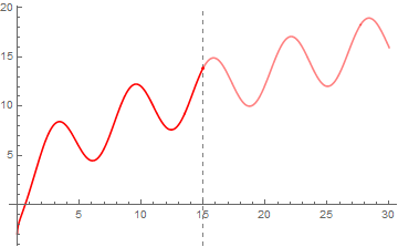
If the same threshold applies to all plots, you can add the options Mesh and MeshShading to p1, p2 and p3 and use the option GridLines in Show:

Note: You might want top play with ConditionalExpression and Piecewise to get all three plots using a single Plot.

An alternative trick is to add a semi-transparent rectangle as Epilog:

With[{a1 = 1, a2 = 2, a = 3, b1 = 1, b2 = 2, b = 3, lag1 = 26, 
  lag = 30, time1 = 40, time2 = 36, time3 = 39}, 
 p1 = Plot[a Sqrt[x] - b Cos[x], {x, 0, time1}];
 p2 = Plot[a1 Sqrt[x] - b1 Cos[x], {x, time1 - lag, time2}, PlotStyle -> Red];
 p3 = Plot[a2 Sqrt[x] - b2 Cos[x], {x, time2 - lag1, time3}, PlotStyle -> Green];
 Show[p1, p2, p3, 
  Epilog -> {Opacity[.8, White], Rectangle[{15, 0}, {40, 40}]}, 
  GridLines -> {{15}, None}, 
  GridLinesStyle -> Directive[Gray, Dashed], PlotRange -> All]]

added 992 characters in body

Source Link

edited Dec 11, 2020 at 20:43

kglr

400.5k
18
488
929

Loading

Source Link

created Dec 11, 2020 at 20:22

kglr

400.5k
18
488
929

Loading

Stack Exchange Network

Return to Answer