added 231 characters in body
Source Link
acl
  • 19.9k
  • 3
  • 66
  • 94

If I define

expr = Function[{a, b},
   Evaluate@withTransforms[intgnd]];

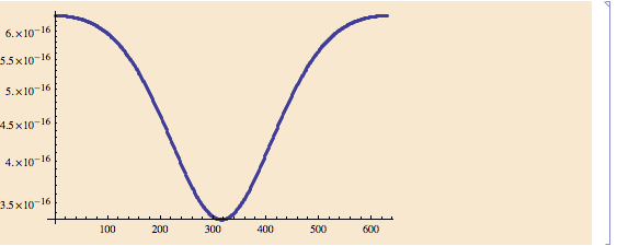
(with intgnd the expression given at the top of the question), I get tiny differences between points symmetric around $b=\pi$:

ListLogPlot[Abs[expr[.3, #] + expr[.3, 2 Pi - #] & /@ Range[0, 2 Pi, .01]]]
Mathematica graphics

so even if your coefficients are accurate, you will have lots of trouble obtaining good results unless you greatly increase working precision (and force the precision of your input numbers to be higher than machine precision).

If you can, it's probably better to rescale your variables at some earlier point to avoid such extreme numbers.

I appreciate that this isn't actually a solution; I'll remove it eventually (this information was too muchOne may also see what is going on as follows:

t={
 NIntegrate[expr[a, b], {a, 0, Pi/4}, {b, 0, Pi}], 
 NIntegrate[expr[a, b], {a, 0, Pi/4}, {b, Pi, 2 Pi}]
 }

(*{-0.0000297965 + 0.000112249 I, 0.0000297965- 0.000112249 I}*)

Plus@@t
(*-2.23895*10^-16 + 1.1891*10^-16 I*)

ie, the two halves are very close to putbeing equal in a comment)magnitude.

If I define

expr = Function[{a, b},
   Evaluate@withTransforms[intgnd]];

(with intgnd the expression given at the top of the question), I get tiny differences between points symmetric around $b=\pi$:

ListLogPlot[Abs[expr[.3, #] + expr[.3, 2 Pi - #] & /@ Range[0, 2 Pi, .01]]]

Mathematica graphics

so even if your coefficients are accurate, you will have lots of trouble obtaining good results unless you greatly increase working precision (and force the precision of your input numbers to be higher than machine precision).

If you can, it's probably better to rescale your variables at some earlier point to avoid such extreme numbers.

I appreciate that this isn't actually a solution; I'll remove it eventually (this information was too much to put in a comment).

If I define

expr = Function[{a, b},
   Evaluate@withTransforms[intgnd]];

(with intgnd the expression given at the top of the question), I get tiny differences between points symmetric around $b=\pi$:

ListLogPlot[Abs[expr[.3, #] + expr[.3, 2 Pi - #] & /@ Range[0, 2 Pi, .01]]]

Mathematica graphics

so even if your coefficients are accurate, you will have lots of trouble obtaining good results unless you greatly increase working precision (and force the precision of your input numbers to be higher than machine precision).

If you can, it's probably better to rescale your variables at some earlier point to avoid such extreme numbers.

One may also see what is going on as follows:

t={
 NIntegrate[expr[a, b], {a, 0, Pi/4}, {b, 0, Pi}], 
 NIntegrate[expr[a, b], {a, 0, Pi/4}, {b, Pi, 2 Pi}]
 }

(*{-0.0000297965 + 0.000112249 I, 0.0000297965- 0.000112249 I}*)

Plus@@t
(*-2.23895*10^-16 + 1.1891*10^-16 I*)

ie, the two halves are very close to being equal in magnitude.

Source Link
acl
  • 19.9k
  • 3
  • 66
  • 94

If I define

expr = Function[{a, b},
   Evaluate@withTransforms[intgnd]];

(with intgnd the expression given at the top of the question), I get tiny differences between points symmetric around $b=\pi$:

ListLogPlot[Abs[expr[.3, #] + expr[.3, 2 Pi - #] & /@ Range[0, 2 Pi, .01]]]

Mathematica graphics

so even if your coefficients are accurate, you will have lots of trouble obtaining good results unless you greatly increase working precision (and force the precision of your input numbers to be higher than machine precision).

If you can, it's probably better to rescale your variables at some earlier point to avoid such extreme numbers.

I appreciate that this isn't actually a solution; I'll remove it eventually (this information was too much to put in a comment).