I have two expressions given by,
$$a = \int_0^1 dx \frac{c z_s^{d+1} x^d}{\sqrt{(1-(z_s/z_h)^{d+1} x^{d+1})(1-c^2 z_s^{2d} x^{2d})}} \tag{1}\label{1},$$
$$S = \int_\epsilon^{z_s} dx \frac{1}{x^d} \sqrt{\frac{1}{(1-(x/z_h)^{d+1})(1-c^2 x^{2d})}}\tag{2}\label{2},$$
where $c=c(z_s)$ is a function of $z_s$, and $a$, $z_h$ are constants which can be given a value later. $d$ is just a dimension parameter which can be given a value say, $d=3$.
The goal is to find an expression of $S$ such that $c$ is eliminated. Now, one condition which can help achieve that is,
$$\frac{dS}{dz_s} = 0\tag{3}\label{3},$$
actually I need to find an expression for the minimal $S$ (with respect to $z_s$) to which $c$ dictates.
I have asked some related problems before but for eq. $\eqref{2}$ in those cases I made a transformation $x=z_sy$ so that the integral limits there is $[\epsilon/z_s,1]$ and then expand out the finite and divergent terms then I just showed the finite terms there so that I allow the lower limit to be 0.
Solving a function inside an integral
Smoothen the result of FindRoot
In this case, I just start with the original integral $\eqref{2}$ and set a small number for $\epsilon$ (this is just a modification of my previous problem in order to eliminate the divergence contribution but the result should not differ for those regions far from the divergence region).
The problem is when I try to plot those same quantities I get a different result.
The previous code,
d = 3;
zh = 1.5;
torootL[a_, c_?NumericQ, z_] := a - NIntegrate[(c z^(d + 1) xd^(d/(d + 1)))/((1 - xd (z/zh)^(d + 1)) (1 - xd^((2 d)/(d + 1)) c^2 (z)^(2 d)))^(1/2), {xd, 0, 1}, MaxRecursion -> 12, PrecisionGoal -> 6, Method -> {"GlobalAdaptive", "SingularityHandler" -> "DoubleExponential"}]
cz[a_?NumericQ, z_?NumericQ] := c /. FindRoot[torootL[a, c, z], {c, 0.001, 0.0000001, 1000}]
intS[a_?NumericQ, z_?NumericQ] := NIntegrate[With[{b = z/zh}, (((-1)/(d - 1)) cz[a, z]^2 z^(2 d)) x^d ((1 - (b x)^(d + 1))/(1 - cz[a, z]^2 (z x)^(2 d)))^(1/2) - ((b^(d + 1) (d + 1))/(2 (d - 1))) x ((1 - cz[a, z]^2 (z x)^(2 d))/(1 - (b x)^(d + 1)))^(1/2) + (b^(d + 1) x)/((1 - (b x)^(d + 1)) (1 - cz[a, z]^2 (z x)^(2 d)))^(1/2)], {x, 0, 1}, MaxRecursion -> 12, PrecisionGoal -> 6, Method -> {"GlobalAdaptive", "SingularityHandler" -> "DoubleExponential"}]
functionS[a_, z_] = ((-((1 - cz[a, z]^2 z^(2 d)) (1 - (z/zh)^(d + 1)))^(1/2)/(d - 1)) + intS[a, z] + 1)/(4 z^(d - 1));
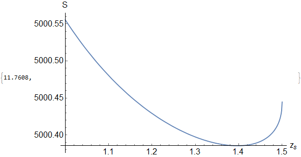
Plot[functionS[0.1, z], {z, 1, zh}, PlotPoints -> 8, AxesLabel -> {"z_s", "S"}, AxesStyle -> Directive[Black, 18], PlotStyle -> Thick, PlotRange -> Full, ImageSize -> Large] // Quiet // AbsoluteTiming
produces this plot,

The present code where I just changed the lines corresponding to the discussion I made above,
d = 3;
zh = 1.5;
torootL[a_, c_?NumericQ, z_] := a - NIntegrate[(c z^(d + 1) xd^(d/(d + 1)))/((1 - xd (z/zh)^(d + 1)) (1 - xd^((2 d)/(d + 1)) c^2 (z)^(2 d)))^(1/2), {xd, 0, 1}, MaxRecursion -> 12, PrecisionGoal -> 6, Method -> {"GlobalAdaptive", "SingularityHandler" -> "DoubleExponential"}]
cz[a_?NumericQ, z_?NumericQ] := c /. FindRoot[torootL[a, c, z], {c, 0.001, 0.0000001, 1000}]

intS[a_?NumericQ, z_?NumericQ] := NIntegrate[(1/x^d) (1/((1 - (x/zh)^(d + 1)) (1 - cz[a, z]^2 x^(2 d))))^(1/2), {x, 10^-10, z}, MaxRecursion -> 20, PrecisionGoal -> 6, Method -> {"GlobalAdaptive"}]
functionS[a_, z_] = intS[a, z] + 1/(z^(d - 1));
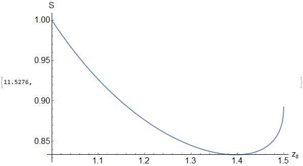
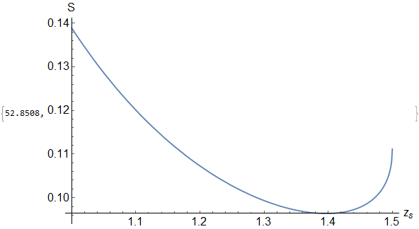
Plot[functionS[0.1, z], {z, 1, zh}, PlotPoints -> 8, AxesLabel -> {"z_s", "S"}, AxesStyle -> Directive[Black, 18], PlotStyle -> Thick, PlotRange -> Automatic, ImageSize -> Large] // Quiet // AbsoluteTiming
produces the plot,

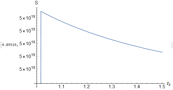
where the Method I used in the present is only GlobalAdaptive since if I use the Method in the old code it produces a flat line which I don't know why. Anyways, the old and present codes should produce the same plot especially in those region close to $z_s = 1.5$ to which in the first image you can see a minimum occurring around $z_s \approx 1.4$.
Why is this so? I'm still trying to understand the NIntegrate Integration Strategies documentation although it is hard to understand for me since I'm not a heavy user maybe until now.
I was thinking of maybe there is a different strategy to eliminate $c$ in the expression for $S$ using $\eqref{1}$ $\eqref{2}$ $\eqref{3}$ at the same time. Any comments?

