added 1 character in body
Source Link
xzczd
  • 68.4k
  • 9
  • 174
  • 489

The integral diverges, please see Michael's answer for more detaldetail. This is just an answer reproducing result of v5.

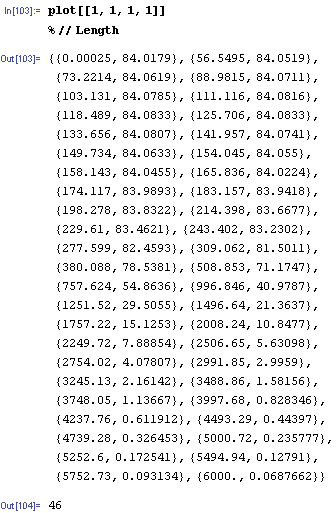
Unlike higher versions, v5 is using very few points for the generation of graphic:

plot = Plot[T, {τ, 0, 6*10^3}]; // AbsoluteTiming
(* {32.1406250 Second, Null} *)

plot[[1, 1, 1, 1]]
% // Length

enter image description here

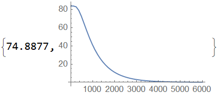
To obtain the result in a reasonable time in higher versions, just limit the points for plotting:

Quiet@Plot[T, {τ, 0, 6*10^3}, MaxRecursion -> 0] // AbsoluteTiming

enter image description here

Still a bit slower than v5, but acceptable in my view.


Update: A More General Solution

The solution above works at least in v12.0.1, v12.1.1 and v11.3, but in v8.0.4 and v9.0.1 samples like

T /. τ -> 1 // AbsoluteTiming

returns unevaluated (to be precise, NIntegrate[…] therein returns unevaluated) after nconv warning generates. If one still needs the result in v5, a possible approach is to implement the "ExtrapolatingOscillatory" method ourselves as I've done here:

Clear[int, separateint]
zero[i_] = Piecewise[{{BesselJZero[0, i], i > 0}}]; 
separateint[f_, t_, i_?NumericQ, prec_] := 
 NIntegrate[BesselJ[0, y] f[y, t], {y, zero@i, zero[i + 1]}, WorkingPrecision -> prec, 
  MaxRecursion -> 40]; 
int[f_, t_?NumericQ, prec_ : MachinePrecision] := 
 NSum[separateint[f, t, i, prec], {i, 0, Infinity}, Method -> "AlternatingSigns", 
  WorkingPrecision -> prec];

The usage of int is as follows:

Clear@func;
func[y_, τ_] = 
  1/Sqrt[(y^2 + w^2)^3]*1/d*(1 - Erf[(p*10^-15 - 1)/Sqrt[2]])*
   Exp[(p*10^-15)^2/2 - p*10^-15*(1 - τ)]*y*w;

T = 10^18*Sqrt[π/2]*int[func, τ];

T /. τ -> 1
(* 84.0182 *)

Plot[T, {τ, 0, 6*10^3}, MaxRecursion -> 0] // AbsoluteTiming

The resulting graphic is the same as shown above, but the solution also works in v8.0.4 and v9.0.1.

This solution also works for the Tc and Td in your new question, on which NIntegrate of v12 again returns unevaluated.

The integral diverges, please see Michael's answer for more detal. This is just an answer reproducing result of v5.

Unlike higher versions, v5 is using very few points for the generation of graphic:

plot = Plot[T, {τ, 0, 6*10^3}]; // AbsoluteTiming
(* {32.1406250 Second, Null} *)

plot[[1, 1, 1, 1]]
% // Length

enter image description here

To obtain the result in a reasonable time in higher versions, just limit the points for plotting:

Quiet@Plot[T, {τ, 0, 6*10^3}, MaxRecursion -> 0] // AbsoluteTiming

enter image description here

Still a bit slower than v5, but acceptable in my view.


Update: A More General Solution

The solution above works at least in v12.0.1, v12.1.1 and v11.3, but in v8.0.4 and v9.0.1 samples like

T /. τ -> 1 // AbsoluteTiming

returns unevaluated (to be precise, NIntegrate[…] therein returns unevaluated) after nconv warning generates. If one still needs the result in v5, a possible approach is to implement the "ExtrapolatingOscillatory" method ourselves as I've done here:

Clear[int, separateint]
zero[i_] = Piecewise[{{BesselJZero[0, i], i > 0}}]; 
separateint[f_, t_, i_?NumericQ, prec_] := 
 NIntegrate[BesselJ[0, y] f[y, t], {y, zero@i, zero[i + 1]}, WorkingPrecision -> prec, 
  MaxRecursion -> 40]; 
int[f_, t_?NumericQ, prec_ : MachinePrecision] := 
 NSum[separateint[f, t, i, prec], {i, 0, Infinity}, Method -> "AlternatingSigns", 
  WorkingPrecision -> prec];

The usage of int is as follows:

Clear@func;
func[y_, τ_] = 
  1/Sqrt[(y^2 + w^2)^3]*1/d*(1 - Erf[(p*10^-15 - 1)/Sqrt[2]])*
   Exp[(p*10^-15)^2/2 - p*10^-15*(1 - τ)]*y*w;

T = 10^18*Sqrt[π/2]*int[func, τ];

T /. τ -> 1
(* 84.0182 *)

Plot[T, {τ, 0, 6*10^3}, MaxRecursion -> 0] // AbsoluteTiming

The resulting graphic is the same as shown above, but the solution also works in v8.0.4 and v9.0.1.

This solution also works for the Tc and Td in your new question, on which NIntegrate of v12 again returns unevaluated.
The integral diverges, please see Michael's answer for more detail. This is just an answer reproducing result of v5.

Unlike higher versions, v5 is using very few points for the generation of graphic:

plot = Plot[T, {τ, 0, 6*10^3}]; // AbsoluteTiming
(* {32.1406250 Second, Null} *)

plot[[1, 1, 1, 1]]
% // Length

enter image description here

To obtain the result in a reasonable time in higher versions, just limit the points for plotting:

Quiet@Plot[T, {τ, 0, 6*10^3}, MaxRecursion -> 0] // AbsoluteTiming

enter image description here

Still a bit slower than v5, but acceptable in my view.


Update: A More General Solution

The solution above works at least in v12.0.1, v12.1.1 and v11.3, but in v8.0.4 and v9.0.1 samples like

T /. τ -> 1 // AbsoluteTiming

returns unevaluated (to be precise, NIntegrate[…] therein returns unevaluated) after nconv warning generates. If one still needs the result in v5, a possible approach is to implement the "ExtrapolatingOscillatory" method ourselves as I've done here:

Clear[int, separateint]
zero[i_] = Piecewise[{{BesselJZero[0, i], i > 0}}]; 
separateint[f_, t_, i_?NumericQ, prec_] := 
 NIntegrate[BesselJ[0, y] f[y, t], {y, zero@i, zero[i + 1]}, WorkingPrecision -> prec, 
  MaxRecursion -> 40]; 
int[f_, t_?NumericQ, prec_ : MachinePrecision] := 
 NSum[separateint[f, t, i, prec], {i, 0, Infinity}, Method -> "AlternatingSigns", 
  WorkingPrecision -> prec];

The usage of int is as follows:

Clear@func;
func[y_, τ_] = 
  1/Sqrt[(y^2 + w^2)^3]*1/d*(1 - Erf[(p*10^-15 - 1)/Sqrt[2]])*
   Exp[(p*10^-15)^2/2 - p*10^-15*(1 - τ)]*y*w;

T = 10^18*Sqrt[π/2]*int[func, τ];

T /. τ -> 1
(* 84.0182 *)

Plot[T, {τ, 0, 6*10^3}, MaxRecursion -> 0] // AbsoluteTiming

The resulting graphic is the same as shown above, but the solution also works in v8.0.4 and v9.0.1.

This solution also works for the Tc and Td in your new question, on which NIntegrate of v12 again returns unevaluated.

added 228 characters in body
Source Link
xzczd
  • 68.4k
  • 9
  • 174
  • 489

The integral diverges, please see Michael's answer for more detal. This is just an answer reproducing result of v5.

Unlike higher versions, v5 is using very few points for the generation of graphic:

plot = Plot[T, {τ, 0, 6*10^3}]; // AbsoluteTiming
(* {32.1406250 Second, Null} *)

plot[[1, 1, 1, 1]]
% // Length

enter image description here

To obtain the result in a reasonable time in higher versions, just limit the points for plotting:

Quiet@Plot[T, {τ, 0, 6*10^3}, MaxRecursion -> 0] // AbsoluteTiming

enter image description here

Still a bit slower than v5, but acceptable in my view.


Update: A More General Solution

The solution above works at least in v12.0.1, v12.1.1 and v11.3, but in v8.0.4 and v9.0.1 samples like

T /. τ -> 1 // AbsoluteTiming

returns unevaluated (to be precise, NIntegrate[…] therein returns unevaluated) after nconv warning generates. If one still needs the result in v5, which looks like a bugpossible approach is to me. So let's implement the "ExtrapolatingOscillatory" method ourselves as I've done here:

Clear[int, separateint]
zero[i_] = Piecewise[{{BesselJZero[0, i], i > 0}}]; 
separateint[f_, t_, i_?NumericQ, prec_] := 
 NIntegrate[BesselJ[0, y] f[y, t], {y, zero@i, zero[i + 1]}, WorkingPrecision -> prec, 
  MaxRecursion -> 40]; 
int[f_, t_?NumericQ, prec_ : MachinePrecision] := 
 NSum[separateint[f, t, i, prec], {i, 0, Infinity}, Method -> "AlternatingSigns", 
  WorkingPrecision -> prec];

The usage of int is as follows:

Clear@func;
func[y_, τ_] = 
  1/Sqrt[(y^2 + w^2)^3]*1/d*(1 - Erf[(p*10^-15 - 1)/Sqrt[2]])*
   Exp[(p*10^-15)^2/2 - p*10^-15*(1 - τ)]*y*w;

T = 10^18*Sqrt[π/2]*int[func, τ];

T /. τ -> 1
(* 84.0182 *)

Plot[T, {τ, 0, 6*10^3}, MaxRecursion -> 0] // AbsoluteTiming

The resulting graphic is the same as shown above, but the solution also works in v8.0.4 and v9.0.1.

This solution also works for the Tc and Td in your new question, on which NIntegrate of v12 failsagain returns unevaluated.

Unlike higher versions, v5 is using very few points for the generation of graphic:

plot = Plot[T, {τ, 0, 6*10^3}]; // AbsoluteTiming
(* {32.1406250 Second, Null} *)

plot[[1, 1, 1, 1]]
% // Length

enter image description here

To obtain the result in a reasonable time in higher versions, just limit the points for plotting:

Quiet@Plot[T, {τ, 0, 6*10^3}, MaxRecursion -> 0] // AbsoluteTiming

enter image description here

Still a bit slower than v5, but acceptable in my view.


Update: A More General Solution

The solution above works at least in v12.0.1, v12.1.1 and v11.3, but in v8.0.4 and v9.0.1 samples like

T /. τ -> 1 // AbsoluteTiming

returns unevaluated (to be precise, NIntegrate[…] therein returns unevaluated) after nconv warning generates, which looks like a bug to me. So let's implement the "ExtrapolatingOscillatory" method ourselves as I've done here:

Clear[int, separateint]
zero[i_] = Piecewise[{{BesselJZero[0, i], i > 0}}]; 
separateint[f_, t_, i_?NumericQ, prec_] := 
 NIntegrate[BesselJ[0, y] f[y, t], {y, zero@i, zero[i + 1]}, WorkingPrecision -> prec, 
  MaxRecursion -> 40]; 
int[f_, t_?NumericQ, prec_ : MachinePrecision] := 
 NSum[separateint[f, t, i, prec], {i, 0, Infinity}, Method -> "AlternatingSigns", 
  WorkingPrecision -> prec];

The usage of int is as follows:

Clear@func;
func[y_, τ_] = 
  1/Sqrt[(y^2 + w^2)^3]*1/d*(1 - Erf[(p*10^-15 - 1)/Sqrt[2]])*
   Exp[(p*10^-15)^2/2 - p*10^-15*(1 - τ)]*y*w;

T = 10^18*Sqrt[π/2]*int[func, τ];

T /. τ -> 1
(* 84.0182 *)

Plot[T, {τ, 0, 6*10^3}, MaxRecursion -> 0] // AbsoluteTiming

The resulting graphic is the same as shown above, but the solution also works in v8.0.4 and v9.0.1.

This solution also works for the Tc and Td in your new question, on which NIntegrate of v12 fails.

The integral diverges, please see Michael's answer for more detal. This is just an answer reproducing result of v5.

Unlike higher versions, v5 is using very few points for the generation of graphic:

plot = Plot[T, {τ, 0, 6*10^3}]; // AbsoluteTiming
(* {32.1406250 Second, Null} *)

plot[[1, 1, 1, 1]]
% // Length

enter image description here

To obtain the result in a reasonable time in higher versions, just limit the points for plotting:

Quiet@Plot[T, {τ, 0, 6*10^3}, MaxRecursion -> 0] // AbsoluteTiming

enter image description here

Still a bit slower than v5, but acceptable in my view.


Update: A More General Solution

The solution above works at least in v12.0.1, v12.1.1 and v11.3, but in v8.0.4 and v9.0.1 samples like

T /. τ -> 1 // AbsoluteTiming

returns unevaluated (to be precise, NIntegrate[…] therein returns unevaluated) after nconv warning generates. If one still needs the result in v5, a possible approach is to implement the "ExtrapolatingOscillatory" method ourselves as I've done here:

Clear[int, separateint]
zero[i_] = Piecewise[{{BesselJZero[0, i], i > 0}}]; 
separateint[f_, t_, i_?NumericQ, prec_] := 
 NIntegrate[BesselJ[0, y] f[y, t], {y, zero@i, zero[i + 1]}, WorkingPrecision -> prec, 
  MaxRecursion -> 40]; 
int[f_, t_?NumericQ, prec_ : MachinePrecision] := 
 NSum[separateint[f, t, i, prec], {i, 0, Infinity}, Method -> "AlternatingSigns", 
  WorkingPrecision -> prec];

The usage of int is as follows:

Clear@func;
func[y_, τ_] = 
  1/Sqrt[(y^2 + w^2)^3]*1/d*(1 - Erf[(p*10^-15 - 1)/Sqrt[2]])*
   Exp[(p*10^-15)^2/2 - p*10^-15*(1 - τ)]*y*w;

T = 10^18*Sqrt[π/2]*int[func, τ];

T /. τ -> 1
(* 84.0182 *)

Plot[T, {τ, 0, 6*10^3}, MaxRecursion -> 0] // AbsoluteTiming

The resulting graphic is the same as shown above, but the solution also works in v8.0.4 and v9.0.1.

This solution also works for the Tc and Td in your new question, on which NIntegrate of v12 again returns unevaluated.

Simplify the code a bit.
Source Link
xzczd
  • 68.4k
  • 9
  • 174
  • 489

Unlike higher versions, v5 is using very few points for the generation of graphic:

plot = Plot[T, {τ, 0, 6*10^3}]; // AbsoluteTiming
(* {32.1406250 Second, Null} *)

plot[[1, 1, 1, 1]]
% // Length

enter image description here

To obtain the result in a reasonable time in higher versions, just limit the points for plotting:

Quiet@Plot[T, {τ, 0, 6*10^3}, MaxRecursion -> 0] // AbsoluteTiming

enter image description here

Still a bit slower than v5, but acceptable in my view.


Update: A More General Solution

The solution above works at least in v12.0.1, v12.1.1 and v11.3, but in v8.0.4 and v9.0.1 samples like

T /. τ -> 1 // AbsoluteTiming

returns unevaluated (to be precise, NIntegrate[…] therein returns unevaluated) after nconv warning generates, which looks like a bug to me. So let's implement the "ExtrapolatingOscillatory" method ourselves as I've done here:

Clear[int, separateint]
zero[i_] = Piecewise[{{BesselJZero[0, i], i > 0}}]; 
separateint[f_, t_, i_?NumericQ, prec_] := 
 NIntegrate[BesselJ[0, y] f[y, t], {y, zero@i, zero[i + 1]}, WorkingPrecision -> prec, 
  MaxRecursion -> 40]; 
int[f_, t_?NumericQ, prec_ : MachinePrecision] := 
 NSum[separateint[f, t, i, prec], {i, 0, Infinity}, Method -> "AlternatingSigns", 
  WorkingPrecision -> prec];

The usage of int is as follows:

Clear@func;
func[y_?NumericQ, τ_?NumericQ]τ_] = 
  1/Sqrt[(y^2 + w^2)^3]*1/d*(1 - Erf[(p*10^-15 - 1)/Sqrt[2]])*
   Exp[(p*10^-15)^2/2 - p*10^-15*(1 - τ)]*y*w;

T = 10^18*Sqrt[π/2]*int[func, τ];

T /. τ -> 1
(* 84.0182 *)

Plot[T, {τ, 0, 6*10^3}, MaxRecursion -> 0] // AbsoluteTiming

The resulting graphic is the same as shown above, but the solution also works in v8.0.4 and v9.0.1.

This solution also works for the Tc and Td in your new question, on which NIntegrate of v12 fails.

Unlike higher versions, v5 is using very few points for the generation of graphic:

plot = Plot[T, {τ, 0, 6*10^3}]; // AbsoluteTiming
(* {32.1406250 Second, Null} *)

plot[[1, 1, 1, 1]]
% // Length

enter image description here

To obtain the result in a reasonable time in higher versions, just limit the points for plotting:

Quiet@Plot[T, {τ, 0, 6*10^3}, MaxRecursion -> 0] // AbsoluteTiming

enter image description here

Still a bit slower than v5, but acceptable in my view.


Update: A More General Solution

The solution above works at least in v12.0.1, v12.1.1 and v11.3, but in v8.0.4 and v9.0.1 samples like

T /. τ -> 1 // AbsoluteTiming

returns unevaluated (to be precise, NIntegrate[…] therein returns unevaluated) after nconv warning generates, which looks like a bug to me. So let's implement the "ExtrapolatingOscillatory" method ourselves as I've done here:

Clear[int, separateint]
zero[i_] = Piecewise[{{BesselJZero[0, i], i > 0}}]; 
separateint[f_, t_, i_?NumericQ, prec_] := 
 NIntegrate[BesselJ[0, y] f[y, t], {y, zero@i, zero[i + 1]}, WorkingPrecision -> prec, 
  MaxRecursion -> 40]; 
int[f_, t_?NumericQ, prec_ : MachinePrecision] := 
 NSum[separateint[f, t, i, prec], {i, 0, Infinity}, Method -> "AlternatingSigns", 
  WorkingPrecision -> prec];

The usage of int is as follows:

Clear@func;
func[y_?NumericQ, τ_?NumericQ] = 
  1/Sqrt[(y^2 + w^2)^3]*1/d*(1 - Erf[(p*10^-15 - 1)/Sqrt[2]])*
   Exp[(p*10^-15)^2/2 - p*10^-15*(1 - τ)]*y*w;

T = 10^18*Sqrt[π/2]*int[func, τ];

T /. τ -> 1
(* 84.0182 *)

Plot[T, {τ, 0, 6*10^3}, MaxRecursion -> 0] // AbsoluteTiming

The resulting graphic is the same as shown above, but the solution also works in v8.0.4 and v9.0.1.

This solution also works for the Tc and Td in your new question, on which NIntegrate of v12 fails.

Unlike higher versions, v5 is using very few points for the generation of graphic:

plot = Plot[T, {τ, 0, 6*10^3}]; // AbsoluteTiming
(* {32.1406250 Second, Null} *)

plot[[1, 1, 1, 1]]
% // Length

enter image description here

To obtain the result in a reasonable time in higher versions, just limit the points for plotting:

Quiet@Plot[T, {τ, 0, 6*10^3}, MaxRecursion -> 0] // AbsoluteTiming

enter image description here

Still a bit slower than v5, but acceptable in my view.


Update: A More General Solution

The solution above works at least in v12.0.1, v12.1.1 and v11.3, but in v8.0.4 and v9.0.1 samples like

T /. τ -> 1 // AbsoluteTiming

returns unevaluated (to be precise, NIntegrate[…] therein returns unevaluated) after nconv warning generates, which looks like a bug to me. So let's implement the "ExtrapolatingOscillatory" method ourselves as I've done here:

Clear[int, separateint]
zero[i_] = Piecewise[{{BesselJZero[0, i], i > 0}}]; 
separateint[f_, t_, i_?NumericQ, prec_] := 
 NIntegrate[BesselJ[0, y] f[y, t], {y, zero@i, zero[i + 1]}, WorkingPrecision -> prec, 
  MaxRecursion -> 40]; 
int[f_, t_?NumericQ, prec_ : MachinePrecision] := 
 NSum[separateint[f, t, i, prec], {i, 0, Infinity}, Method -> "AlternatingSigns", 
  WorkingPrecision -> prec];

The usage of int is as follows:

Clear@func;
func[y_, τ_] = 
  1/Sqrt[(y^2 + w^2)^3]*1/d*(1 - Erf[(p*10^-15 - 1)/Sqrt[2]])*
   Exp[(p*10^-15)^2/2 - p*10^-15*(1 - τ)]*y*w;

T = 10^18*Sqrt[π/2]*int[func, τ];

T /. τ -> 1
(* 84.0182 *)

Plot[T, {τ, 0, 6*10^3}, MaxRecursion -> 0] // AbsoluteTiming

The resulting graphic is the same as shown above, but the solution also works in v8.0.4 and v9.0.1.

This solution also works for the Tc and Td in your new question, on which NIntegrate of v12 fails.

Add a more general solution.
Source Link
xzczd
  • 68.4k
  • 9
  • 174
  • 489
Loading
added 113 characters in body
Source Link
xzczd
  • 68.4k
  • 9
  • 174
  • 489
Loading
added 9 characters in body
Source Link
xzczd
  • 68.4k
  • 9
  • 174
  • 489
Loading
added 243 characters in body
Source Link
xzczd
  • 68.4k
  • 9
  • 174
  • 489
Loading
added 3 characters in body
Source Link
xzczd
  • 68.4k
  • 9
  • 174
  • 489
Loading
Source Link
xzczd
  • 68.4k
  • 9
  • 174
  • 489
Loading