Return to Question

I am having a bit of trouble when it comes to plotting the solution of a system of non-linear ODE's.

I write

pfun = ParametricNDSolveValue[
  system, {x[t], y[t], z[t], px[t], py[t], pz[t]}, {t, 0, 1}, {tau, 
   omega, xi, yi, zi, pxi, pyi, pzi}]

• xi, yi, zi, pxi, pyi, pzi are the initial conditions

• tau and omega are just two other parameters

This gives me a single parametric function as the output.

I then write

Manipulate[
 Plot[pfun[tau0, omega0, xi0, yi0, zi0, pxi0, pyi0, pzi0], {t, 0, 
   1}], {{tau0, 0.5, "strength"}, 0, 1}, {{omega0, 2 Pi}, 0, 
  2 Pi}, {{xi0, 1, "initial theta"}, 0, Pi}, {{yi0, 1, "initial phi"},
   0, 2 Pi}, {{zi0, 1 , "initial phase"}, 0, 2 Pi}, {{pxi0, 1}, -Pi , 
  Pi}, {{pyi0, 1}, -Pi, Pi}, {{pzi0, 1}, -Pi, Pi}]

Which does correctly plot a bunch of solutions, with parameters that I can vary, however, I cannot then make the different plots show up in different colours!

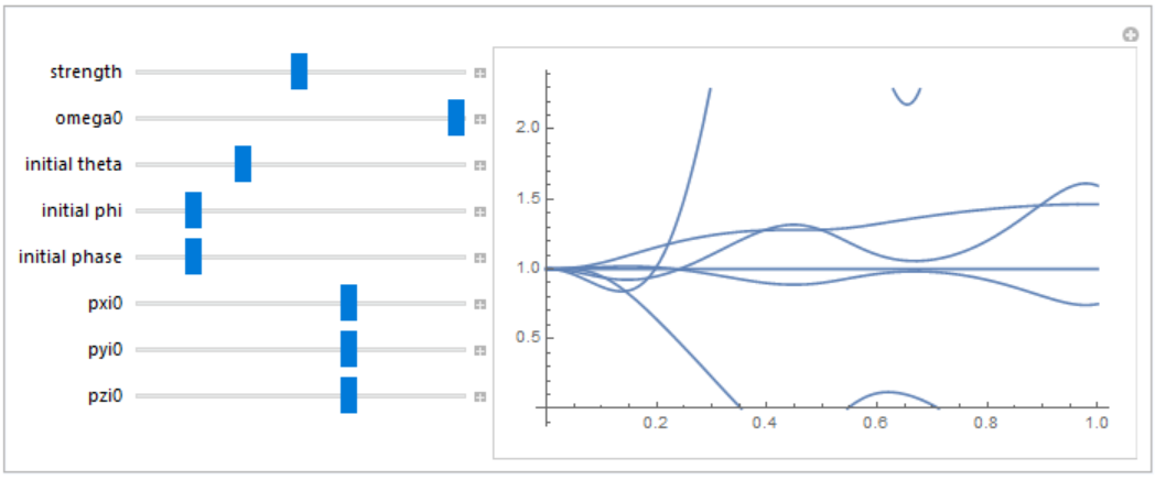
Could anyone explain what I need to do?

I have tried to use things like "Plot Style" in the third argument of the "Plot" function, but this does not work.

Edit:

I will copy and paste a full simple example that causes me the same issue as described above.

$Assumptions = {x, y, tau, xi, yi} \[Element] Reals

system = {D[x[t], t] == (Cos[x[t]] y[t])/tau, 
  D[y[t], t] == (Sin[y[t]] x[t])/tau, x[0] == xi, y[0] == yi}

pfun = ParametricNDSolveValue[
  system, {x[t], y[t]}, {t, 0, 1}, {tau, xi, yi}]

Manipulate[
 Plot[pfun[tau0, xi0, yi0], {t, 0, 1}], {{tau0, 0.5, "strength"}, 0, 
  1}, {{xi0, 1, "initial theta"}, 0, 
  Pi}, {{yi0, 1, "initial phi"}, 0, 2 Pi}]

I am having a bit of trouble when it comes to plotting the solution of a system of non-linear ODE's.

I write

pfun = ParametricNDSolveValue[
  system, {x[t], y[t], z[t], px[t], py[t], pz[t]}, {t, 0, 1}, {tau, 
   omega, xi, yi, zi, pxi, pyi, pzi}]

• xi, yi, zi, pxi, pyi, pzi are the initial conditions

• tau and omega are just two other parameters

This gives me a single parametric function as the output.

I then write

Manipulate[
 Plot[pfun[tau0, omega0, xi0, yi0, zi0, pxi0, pyi0, pzi0], {t, 0, 
   1}], {{tau0, 0.5, "strength"}, 0, 1}, {{omega0, 2 Pi}, 0, 
  2 Pi}, {{xi0, 1, "initial theta"}, 0, Pi}, {{yi0, 1, "initial phi"},
   0, 2 Pi}, {{zi0, 1 , "initial phase"}, 0, 2 Pi}, {{pxi0, 1}, -Pi , 
  Pi}, {{pyi0, 1}, -Pi, Pi}, {{pzi0, 1}, -Pi, Pi}]

Which does correctly plot a bunch of solutions, with parameters that I can vary, however, I cannot then make the different plots show up in different colours!

Could anyone explain what I need to do?

I have tried to use things like "Plot Style" in the third argument of the "Plot" function, but this does not work.

Edit:

I will copy and paste a full simple example that causes me the same issue as described above.

$Assumptions = {x, y, tau, xi, yi} ∈ Reals

system = {D[x[t], t] == (Cos[x[t]] y[t])/tau, 
  D[y[t], t] == (Sin[y[t]] x[t])/tau, x[0] == xi, y[0] == yi}

pfun = ParametricNDSolveValue[
  system, {x[t], y[t]}, {t, 0, 1}, {tau, xi, yi}]

Manipulate[
 Plot[pfun[tau0, xi0, yi0], {t, 0, 1}], {{tau0, 0.5, "strength"}, 0, 
  1}, {{xi0, 1, "initial theta"}, 0, 
  Pi}, {{yi0, 1, "initial phi"}, 0, 2 Pi}]

I am having a bit of trouble when it comes to plotting the solution of a system of non-linear ODE's.

I write

pfun = ParametricNDSolveValue[
  system, {x[t], y[t], z[t], px[t], py[t], pz[t]}, {t, 0, 1}, {tau, 
   omega, xi, yi, zi, pxi, pyi, pzi}]

• xi, yi, zi, pxi, pyi, pzi are the initial conditions

• tau and omega are just two other parameters

This gives me a single parametric function as the output.

I then write

Manipulate[
 Plot[pfun[tau0, omega0, xi0, yi0, zi0, pxi0, pyi0, pzi0], {t, 0, 
   1}], {{tau0, 0.5, "strength"}, 0, 1}, {{omega0, 2 Pi}, 0, 
  2 Pi}, {{xi0, 1, "initial theta"}, 0, Pi}, {{yi0, 1, "initial phi"},
   0, 2 Pi}, {{zi0, 1 , "initial phase"}, 0, 2 Pi}, {{pxi0, 1}, -Pi , 
  Pi}, {{pyi0, 1}, -Pi, Pi}, {{pzi0, 1}, -Pi, Pi}]

Which does correctly plot a bunch of solutions, with parameters that I can vary, however, I cannot then make the different plots show up in different colours!

Could anyone explain what I need to do?

I have tried to use things like "Plot Style" in the third argument of the "Plot" function, but this does not work.

Edit:

I will copy and paste a full simple example that causes me the same issue as described above.

$Assumptions = {x, y, tau, xi, yi} \[Element] Reals

system = {D[x[t], t] == (Cos[x[t]] y[t])/tau, 
  D[y[t], t] == (Sin[y[t]] x[t])/tau, x[0] == xi, y[0] == yi}

pfun = ParametricNDSolveValue[
  system, {x[t], y[t]}, {t, 0, 1}, {tau, xi, yi}]

Manipulate[
 Plot[pfun[tau0, xi0, yi0], {t, 0, 1}], {{tau0, 0.5, "strength"}, 0, 
  1}, {{xi0, 1, "initial theta"}, 0, 
  Pi}, {{yi0, 1, "initial phi"}, 0, 2 Pi}]

I am having a bit of trouble when it comes to plotting the solution of a system of non-linear ODE's.

I write

pfun = ParametricNDSolveValue[
  system, {x[t], y[t], z[t], px[t], py[t], pz[t]}, {t, 0, 1}, {tau, 
   omega, xi, yi, zi, pxi, pyi, pzi}]

• xi, yi, zi, pxi, pyi, pzi are the initial conditions

• tau and omega are just two other parameters

This gives me a single parametric function as the output.

I then write

Manipulate[
 Plot[pfun[tau0, omega0, xi0, yi0, zi0, pxi0, pyi0, pzi0], {t, 0, 
   1}], {{tau0, 0.5, "strength"}, 0, 1}, {{omega0, 2 Pi}, 0, 
  2 Pi}, {{xi0, 1, "initial theta"}, 0, Pi}, {{yi0, 1, "initial phi"},
   0, 2 Pi}, {{zi0, 1 , "initial phase"}, 0, 2 Pi}, {{pxi0, 1}, -Pi , 
  Pi}, {{pyi0, 1}, -Pi, Pi}, {{pzi0, 1}, -Pi, Pi}]

Which does correctly plot a bunch of solutions, with parameters that I can vary, however, I cannot then make the different plots show up in different colours!

Could anyone explain what I need to do?

I have tried to use things like "Plot Style" in the third argument of the "Plot" function, but this does not work.

Edit:

I will copy and paste a full simple example that causes me the same issue as described above.

$Assumptions = {x, y, tau, xi, yi} \[Element] Reals

system = {D[x[t], t] == (Cos[x[t]] y[t])/tau, 
  D[y[t], t] == (Sin[y[t]] x[t])/tau, x[0] == xi, y[0] == yi}

pfun = ParametricNDSolveValue[
  system, {x[t], y[t]}, {t, 0, 1}, {tau, xi, yi}]

Manipulate[
 Plot[pfun[tau0, xi0, yi0], {t, 0, 1}], {{tau0, 0.5, "strength"}, 0, 
  1}, {{xi0, 1, "initial theta"}, 0, 
  Pi}, {{yi0, 1, "initial phi"}, 0, 2 Pi}]

I am having a bit of trouble when it comes to plotting the solution of a system of non-linear ODE's.

I write

pfun = ParametricNDSolveValue[
  system, {x[t], y[t], z[t], px[t], py[t], pz[t]}, {t, 0, 1}, {tau, 
   omega, xi, yi, zi, pxi, pyi, pzi}]

• xi, yi, zi, pxi, pyi, pzi are the initial conditions

• tau and omega are just two other parameters

This gives me a single parametric function as the output.

I then write

Manipulate[
 Plot[pfun[tau0, omega0, xi0, yi0, zi0, pxi0, pyi0, pzi0], {t, 0, 
   1}], {{tau0, 0.5, "strength"}, 0, 1}, {{omega0, 2 Pi}, 0, 
  2 Pi}, {{xi0, 1, "initial theta"}, 0, Pi}, {{yi0, 1, "initial phi"},
   0, 2 Pi}, {{zi0, 1 , "initial phase"}, 0, 2 Pi}, {{pxi0, 1}, -Pi , 
  Pi}, {{pyi0, 1}, -Pi, Pi}, {{pzi0, 1}, -Pi, Pi}]

Which does correctly plot a bunch of solutions, with parameters that I can vary, however, I cannot then make the different plots show up in different colours!

Could anyone explain what I need to do?

I have tried to use things like "Plot Style" in the third argument of the "Plot" function, but this does not work.

I am having a bit of trouble when it comes to plotting the solution of a system of non-linear ODE's.

I write

pfun = ParametricNDSolveValue[
  system, {x[t], y[t], z[t], px[t], py[t], pz[t]}, {t, 0, 1}, {tau, 
   omega, xi, yi, zi, pxi, pyi, pzi}]

• xi, yi, zi, pxi, pyi, pzi are the initial conditions

• tau and omega are just two other parameters

This gives me a single parametric function as the output.

I then write

Manipulate[
 Plot[pfun[tau0, omega0, xi0, yi0, zi0, pxi0, pyi0, pzi0], {t, 0, 
   1}], {{tau0, 0.5, "strength"}, 0, 1}, {{omega0, 2 Pi}, 0, 
  2 Pi}, {{xi0, 1, "initial theta"}, 0, Pi}, {{yi0, 1, "initial phi"},
   0, 2 Pi}, {{zi0, 1 , "initial phase"}, 0, 2 Pi}, {{pxi0, 1}, -Pi , 
  Pi}, {{pyi0, 1}, -Pi, Pi}, {{pzi0, 1}, -Pi, Pi}]

Which does correctly plot a bunch of solutions, with parameters that I can vary, however, I cannot then make the different plots show up in different colours!

Could anyone explain what I need to do?

I have tried to use things like "Plot Style" in the third argument of the "Plot" function, but this does not work.

Edit:

I will copy and paste a full simple example that causes me the same issue as described above.

$Assumptions = {x, y, tau, xi, yi} \[Element] Reals

system = {D[x[t], t] == (Cos[x[t]] y[t])/tau, 
  D[y[t], t] == (Sin[y[t]] x[t])/tau, x[0] == xi, y[0] == yi}

pfun = ParametricNDSolveValue[
  system, {x[t], y[t]}, {t, 0, 1}, {tau, xi, yi}]

Manipulate[
 Plot[pfun[tau0, xi0, yi0], {t, 0, 1}], {{tau0, 0.5, "strength"}, 0, 
  1}, {{xi0, 1, "initial theta"}, 0, 
  Pi}, {{yi0, 1, "initial phi"}, 0, 2 Pi}]