deleted 26 characters in body
Source Link
kirma
  • 19.1k
  • 1
  • 55
  • 95

Here's a quick-and-dirty approach which might be helpful - but is pretty slow on reasonable image sizes (that is, could be improved):

With[{bc = 
    BinCounts[ReIm@data, 
     Sequence @@ ({#1, #2, (#2 - #1)/256} & @@@ 
        CoordinateBounds@ReIm@data)]}, 
  bc /. Map[
    Evaluate[# -> 
       ColorData["SunsetColors"]@
        N@CDF[HistogramDistribution[Flatten@bc]N@CDF[HistogramDistribution@Flatten@bc, #] &], 
    Union@Flatten@bc]] // Image

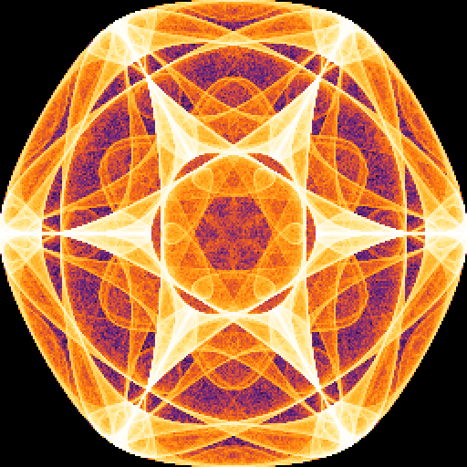
enter image description hereHistogram-based

BinCounts is performed for a square defined by bounds of the dataset and color is assigned to each unique value in the count on basis of CDF of the distribution of these values. In this case ColorData["SunsetColors"] is used as a palette, but something custom could be used as well.

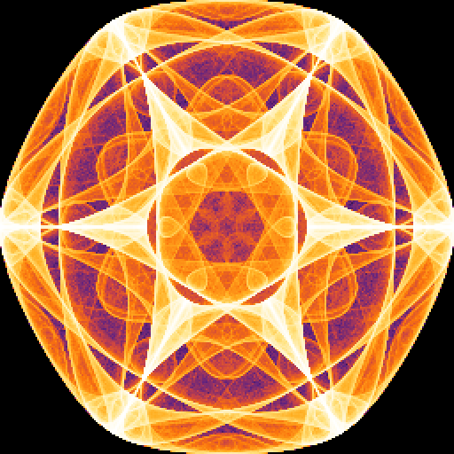
Something similar can be also achieved by "gamma-correcting" the range of bin counts. This is dramatically faster for a reason or another:

With[{bc = 
    BinCounts[ReIm@data, 
     Sequence @@ ({#1, #2, (#2 - #1)/256} & @@@ 
        CoordinateBounds@ReIm@data)]}, 
  Map[
   ColorData["SunsetColors"],
   (bc/N@Max@Flatten@bc)^(1/5), {2}]] // Image

enter image description hereGamma corrected

Here's a quick-and-dirty approach which might be helpful - but is pretty slow on reasonable image sizes (that is, could be improved):

With[{bc = 
    BinCounts[ReIm@data, 
     Sequence @@ ({#1, #2, (#2 - #1)/256} & @@@ 
        CoordinateBounds@ReIm@data)]}, 
  bc /. Map[
    Evaluate[# -> 
       ColorData["SunsetColors"]@
        N@CDF[HistogramDistribution[Flatten@bc], #] &], 
    Union@Flatten@bc]] // Image

enter image description here

BinCounts is performed for a square defined by bounds of the dataset and color is assigned to each unique value in the count on basis of CDF of the distribution of these values. In this case ColorData["SunsetColors"] is used as a palette, but something custom could be used as well.

Something similar can be also achieved by "gamma-correcting" the range of bin counts. This is dramatically faster for a reason or another:

With[{bc = 
    BinCounts[ReIm@data, 
     Sequence @@ ({#1, #2, (#2 - #1)/256} & @@@ 
        CoordinateBounds@ReIm@data)]}, 
  Map[
   ColorData["SunsetColors"],
   (bc/N@Max@Flatten@bc)^(1/5), {2}]] // Image
enter image description here

Here's a quick-and-dirty approach which might be helpful - but is pretty slow on reasonable image sizes (that is, could be improved):

With[{bc = 
    BinCounts[ReIm@data, 
     Sequence @@ ({#1, #2, (#2 - #1)/256} & @@@ 
        CoordinateBounds@ReIm@data)]}, 
  bc /. Map[
    Evaluate[# -> 
       ColorData["SunsetColors"]@
        N@CDF[HistogramDistribution@Flatten@bc, #] &], 
    Union@Flatten@bc]] // Image

Histogram-based

BinCounts is performed for a square defined by bounds of the dataset and color is assigned to each unique value in the count on basis of CDF of the distribution of these values. In this case ColorData["SunsetColors"] is used as a palette, but something custom could be used as well.

Something similar can be also achieved by "gamma-correcting" the range of bin counts. This is dramatically faster for a reason or another:

With[{bc = 
    BinCounts[ReIm@data, 
     Sequence @@ ({#1, #2, (#2 - #1)/256} & @@@ 
        CoordinateBounds@ReIm@data)]}, 
  Map[
   ColorData["SunsetColors"],
   (bc/N@Max@Flatten@bc)^(1/5), {2}]] // Image
Gamma corrected

added 477 characters in body
Source Link
kirma
  • 19.1k
  • 1
  • 55
  • 95

Here's a quick-and-dirty approach which might be helpful - but is pretty slow on reasonable image sizes (that is, could be improved):

With[{bc = 
    BinCounts[ReIm@data, 
     Sequence @@ ({#1, #2, (#2 - #1)/256} & @@@ 
        CoordinateBounds@ReIm@data)]}, 
  bc /. Map[
    Evaluate[# -> 
       ColorData["SunsetColors"]@
        N@CDF[HistogramDistribution[Flatten@bc], #] &], 
    Union@Flatten@bc]] // Image

enter image description here

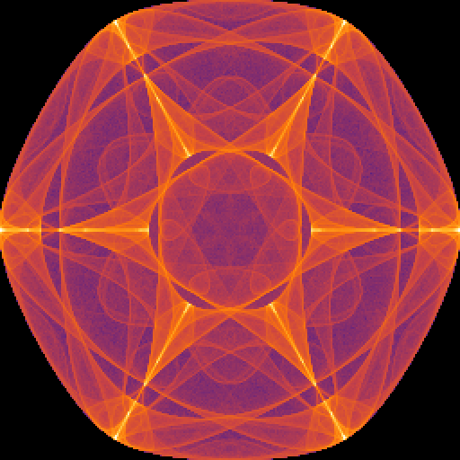
BinCounts is performed for a square defined by bounds of the dataset and color is assigned to each unique value in the count on basis of CDF of the distribution of these values. In this case ColorData["SunsetColors"] is used as a palette, but something custom could be used as well.

Something similar can be also achieved by "gamma-correcting" the range of bin counts. This is dramatically faster for a reason or another:

With[{bc = 
    BinCounts[ReIm@data, 
     Sequence @@ ({#1, #2, (#2 - #1)/256} & @@@ 
        CoordinateBounds@ReIm@data)]}, 
  Map[
   ColorData["SunsetColors"],
   (bc/N@Max@Flatten@bc)^(1/5), {2}]] // Image
enter image description here

Here's a quick-and-dirty approach which might be helpful - but is pretty slow on reasonable image sizes (that is, could be improved):

With[{bc = 
    BinCounts[ReIm@data, 
     Sequence @@ ({#1, #2, (#2 - #1)/256} & @@@ 
        CoordinateBounds@ReIm@data)]}, 
  bc /. Map[
    Evaluate[# -> 
       ColorData["SunsetColors"]@
        N@CDF[HistogramDistribution[Flatten@bc], #] &], 
    Union@Flatten@bc]] // Image

enter image description here

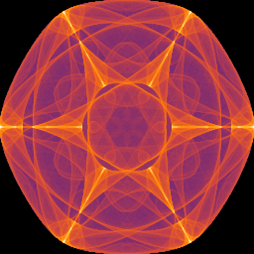
BinCounts is performed for a square defined by bounds of the dataset and color is assigned to each unique value in the count on basis of CDF of the distribution of these values. In this case ColorData["SunsetColors"] is used as a palette, but something custom could be used as well.

Something similar can be also achieved by "gamma-correcting" the range of bin counts. This is dramatically faster for a reason or another:

With[{bc = 
    BinCounts[ReIm@data, 
     Sequence @@ ({#1, #2, (#2 - #1)/256} & @@@ 
        CoordinateBounds@ReIm@data)]}, 
  Map[
   ColorData["SunsetColors"],
   (bc/N@Max@Flatten@bc)^(1/5), {2}]] // Image
enter image description here

Source Link
kirma
  • 19.1k
  • 1
  • 55
  • 95

Here's a quick-and-dirty approach which might be helpful - but is pretty slow on reasonable image sizes (that is, could be improved):

With[{bc = 
    BinCounts[ReIm@data, 
     Sequence @@ ({#1, #2, (#2 - #1)/256} & @@@ 
        CoordinateBounds@ReIm@data)]}, 
  bc /. Map[
    Evaluate[# -> 
       ColorData["SunsetColors"]@
        N@CDF[HistogramDistribution[Flatten@bc], #] &], 
    Union@Flatten@bc]] // Image

enter image description here

BinCounts is performed for a square defined by bounds of the dataset and color is assigned to each unique value in the count on basis of CDF of the distribution of these values. In this case ColorData["SunsetColors"] is used as a palette, but something custom could be used as well.