Return to Answer

FINAL EDIT

k2 = Rationalize[0.000194519, 0];
ϵ = 10^-4; R = Rationalize[1.5472, 0];
j = .00001271;

s1 = ParametricNDSolveValue[{y''[r] + 2 y'[r]/r == k2 Sinh[y[r]], 
    y[ϵ] == y0, y'[ϵ] == 0, 
    WhenEvent[r == 1, y'[r] -> y'[r] + 160/h 0.0714/h1]}, {y, 
    y'}, {r, ϵ, R}, {y0, h, h1}, 
   Method -> "StiffnessSwitching", WorkingPrecision -> 30];

s2[y0_?NumericQ, h_?NumericQ, h1_?NumericQ] := Last[s1[y0, h, h1]]
ff[h_?NumericQ, h1_?NumericQ] := 
 y0 /. FindRoot[s2[y0, h, h1][R], {y0, -10}]
ll[h_?NumericQ, h1_?NumericQ] := 
 4 π j NIntegrate[
   r^2 Exp[-First[s1[ff[h, h1], h, h1]][r]], {r, 0, R}]

To speed-up computation (FindRoot and NIntegrate are very expensive for continuous plotting) I suggest using Interpolation of ll:

llinterp = 
 Interpolation[
  Flatten[Table[{{h, h1}, ll[h, h1]}, {h, 2, 5, 0.1}, {h1, 2, 5, 
     0.1}], 1]]

Now we can define p1 and p2 via llinterp (as of last comment of OP):

p1 = 10 h - llinterp[h, h1] + u
p2 = -u + 10 h1 llinterp[h, h1]

and see what are ContourPlot3Ds:

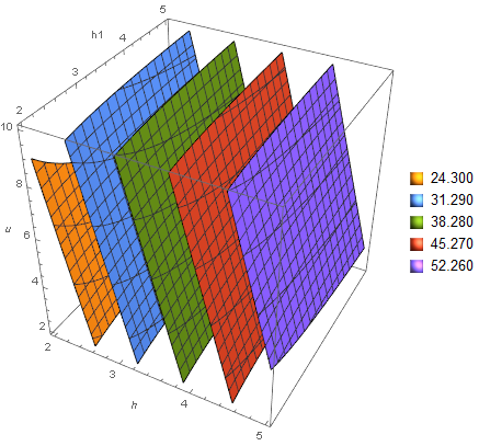
ContourPlot3D[p1, {h, 2, 5}, {h1, 2, 5}, {u, 2, 10}, Contours -> 5, 
PlotLegends -> Automatic, AxesLabel -> {h, h1, u}]

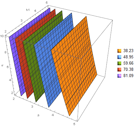
ContourPlot3D[p2, {h, 2, 5}, {h1, 2, 5}, {u, 2, 10}, Contours -> 5, 
PlotLegends -> Automatic, AxesLabel -> {h, h1, u}]

Colors in lenends correspond to values of p1, p2.

Apparently, with given ranges of variables (h, h1, u) we can not fulfil conditions p1 = 0 and p2 = 0. Moreover, these conditions are conflicting: to decreese p1 one has to decrease h, but for p2 situation is opposite. So, OP should think about conditions and/or variables' ranges.

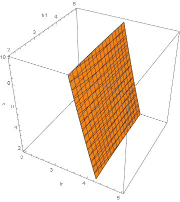
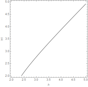
We can also plot intersection (p1 == p2):

ContourPlot3D[p1 == p2, {h, 2, 5}, {h1, 2, 5}, {u, 2, 10}, 
AxesLabel -> {h, h1, u}]

s1 = ParametricNDSolveValue[{y''[r] + 2 y'[r]/r == k2 Sinh[y[r]], 
        y[ϵ] == y0, y'[ϵ] == 0, 
        WhenEvent[r == 1, y'[r] -> y'[r] + 160/h 0.0714/h1]}, {y, 
        y'}, {r, ϵ, R}, {y0, h, h1}, 
       Method -> "StiffnessSwitching", WorkingPrecision -> 30];

s2[y0_?NumericQ, h_?NumericQ, h1_?NumericQ] := Last[s1[y0, h, h1]]
ff[h_, h1_] := y0 /. FindRoot[s2[y0, h, h1][R], {y0, -10}]
ll[h_, h1_] := 4 π j NIntegrate[r^2 Exp[-First[s1[ff[h, h1], h, h1]][r]],{r, 0, R}]

s1 = ParametricNDSolveValue[{y''[r] + 2 y'[r]/r == k2 Sinh[y[r]], 
        y[ϵ] == y0, y'[ϵ] == 0, 
        WhenEvent[r == 1, y'[r] -> y'[r] + 160/h 0.0714/h1]}, {y, 
        y'}, {r, ϵ, R}, {y0, h, h1}, 
       Method -> "StiffnessSwitching", WorkingPrecision -> 30];

s2[y0_?NumericQ, h_?NumericQ, h1_?NumericQ] := Last[s1[y0, h, h1]]
ff[h_?NumericQ, h1_?NumericQ] := y0 /. FindRoot[s2[y0, h, h1][R], {y0, -10}]
ll[h_?NumericQ, h1_?NumericQ] := 4 π j NIntegrate[r^2 Exp[-First[s1[ff[h, h1], h, h1]][r]],{r, 0, R}]

EDIT

To answer additional request: z = 160/h, g = 0.0714/h1. Make corresponding changes:

s1 = ParametricNDSolveValue[{y''[r] + 2 y'[r]/r == k2 Sinh[y[r]], 
        y[ϵ] == y0, y'[ϵ] == 0, 
        WhenEvent[r == 1, y'[r] -> y'[r] + 160/h 0.0714/h1]}, {y, 
        y'}, {r, ϵ, R}, {y0, h, h1}, 
       Method -> "StiffnessSwitching", WorkingPrecision -> 30];

s2[y0_?NumericQ, h_?NumericQ, h1_?NumericQ] := Last[s1[y0, h, h1]]
ff[h_, h1_] := y0 /. FindRoot[s2[y0, h, h1][R], {y0, -10}]
ll[h_, h1_] := 4 π j NIntegrate[r^2 Exp[-First[s1[ff[h, h1], h, h1]][r]],{r, 0, R}]

Now we are ready to plot contour of 10 h - ll[h, h1] - 10 h1 == 0:

ListContourPlot[
 Flatten[Table[{h, h1, 10 h - ll[h, h1] - 10 h1}, {h, 2, 5, 0.1}, {h1,
     2, 5, 0.1}], 1], Contours -> {0}, ContourShading -> None, 
 ContourStyle -> Thick, FrameLabel -> {h, h1}, BaseStyle -> 12]