edited body
Source Link
xzczd
  • 68.4k
  • 9
  • 174
  • 489

You're almost there, I think the main trouble you're facing is that you're not yet familiar enough with list manipulation of Mathematica. Check carefully about how I modify the code:

int[expr_, {t_, L_, R_, step_}] := step*Total[Table[exprstep Total[Table[expr, {t, L + step, R, step}]]

step = 1/100;
bL = 0; bR = 2;
grid = Table[i, {i, bL, bR, step}];

eq = {y1''[t] + t^2 y1[t] - y2''[t] - ((2 + t^2) E^t - t - Cos[t] + Sin[t]), 
      4 t^3 y1'[t] + 6 t^2 y1[t] + 
       y2'''[t] - (Sin[t] - (1 + 2 t) Cos[t] + E^t (1 + 6 t^2 + 4 t^3) + t - 1)};


kernel11 = int[(t - x) y1[x] + y2[x], {x, 0, t}];
kernel21 = int[y1[x] + (t + x) y2[x], {x, 0, t}];

bc = {y1[0] == 1, y1'[0] == 1, y2[0] == 0, y2'[0] == 1, y2''[0] == 0};

kernelSet11 = Table[kernel11, {t, bL, bR, step}] /. {x, bL, a_} :> {x, bL, a, step};
kernelSet21 = Table[kernel21, {t, bL, bR, step}] /. {x, bL, a_} :> {x, bL, a, step};
difforder = 4;
ptoafunc = pdetoae[{y1[t], y2[t]}, grid, difforder];
fullae = ptoafunc[eq] + {kernelSet11, kernelSet21};
aebc = ptoafunc[bc];

{blst, mat} = 
  CoefficientArrays[Flatten[{fullae, aebc}], Flatten[{y1 /@ grid, y2 /@ grid}]];
sollst = LeastSquares[N[mat], -blst];

{sol1, sol2} = ListInterpolation[#, grid] & /@ Partition[sollst, Length@grid];

Plot[{E^y1, sol1[y1]}, {y1, 0, bR}, PlotRange -> All, 
 PlotStyle -> {Automatic, {Red, Dashed}}]
Plot[{Sin[y2], sol2[y2]}, {y2, 0, bR}, PlotRange -> All, 
 PlotStyle -> {Automatic, {Red, Dashed}}]

enter image description here

You're almost there, I think the main trouble you're facing is that you're not yet familiar enough with list manipulation of Mathematica. Check carefully about how I modify the code:

int[expr_, {t_, L_, R_, step_}] := step*Total[Table[expr, {t, L + step, R, step}]]

step = 1/100;
bL = 0; bR = 2;
grid = Table[i, {i, bL, bR, step}];

eq = {y1''[t] + t^2 y1[t] - y2''[t] - ((2 + t^2) E^t - t - Cos[t] + Sin[t]), 
      4 t^3 y1'[t] + 6 t^2 y1[t] + 
       y2'''[t] - (Sin[t] - (1 + 2 t) Cos[t] + E^t (1 + 6 t^2 + 4 t^3) + t - 1)};


kernel11 = int[(t - x) y1[x] + y2[x], {x, 0, t}];
kernel21 = int[y1[x] + (t + x) y2[x], {x, 0, t}];

bc = {y1[0] == 1, y1'[0] == 1, y2[0] == 0, y2'[0] == 1, y2''[0] == 0};

kernelSet11 = Table[kernel11, {t, bL, bR, step}] /. {x, bL, a_} :> {x, bL, a, step};
kernelSet21 = Table[kernel21, {t, bL, bR, step}] /. {x, bL, a_} :> {x, bL, a, step};
difforder = 4;
ptoafunc = pdetoae[{y1[t], y2[t]}, grid, difforder];
fullae = ptoafunc[eq] + {kernelSet11, kernelSet21};
aebc = ptoafunc[bc];

{blst, mat} = 
  CoefficientArrays[Flatten[{fullae, aebc}], Flatten[{y1 /@ grid, y2 /@ grid}]];
sollst = LeastSquares[N[mat], -blst];

{sol1, sol2} = ListInterpolation[#, grid] & /@ Partition[sollst, Length@grid];

Plot[{E^y1, sol1[y1]}, {y1, 0, bR}, PlotRange -> All, 
 PlotStyle -> {Automatic, {Red, Dashed}}]
Plot[{Sin[y2], sol2[y2]}, {y2, 0, bR}, PlotRange -> All, 
 PlotStyle -> {Automatic, {Red, Dashed}}]
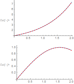
enter image description here

You're almost there, I think the main trouble you're facing is that you're not yet familiar enough with list manipulation of Mathematica. Check carefully about how I modify the code:

int[expr_, {t_, L_, R_, step_}] := step Total[Table[expr, {t, L + step, R, step}]]

step = 1/100;
bL = 0; bR = 2;
grid = Table[i, {i, bL, bR, step}];

eq = {y1''[t] + t^2 y1[t] - y2''[t] - ((2 + t^2) E^t - t - Cos[t] + Sin[t]), 
      4 t^3 y1'[t] + 6 t^2 y1[t] + 
       y2'''[t] - (Sin[t] - (1 + 2 t) Cos[t] + E^t (1 + 6 t^2 + 4 t^3) + t - 1)};


kernel11 = int[(t - x) y1[x] + y2[x], {x, 0, t}];
kernel21 = int[y1[x] + (t + x) y2[x], {x, 0, t}];

bc = {y1[0] == 1, y1'[0] == 1, y2[0] == 0, y2'[0] == 1, y2''[0] == 0};

kernelSet11 = Table[kernel11, {t, bL, bR, step}] /. {x, bL, a_} :> {x, bL, a, step};
kernelSet21 = Table[kernel21, {t, bL, bR, step}] /. {x, bL, a_} :> {x, bL, a, step};
difforder = 4;
ptoafunc = pdetoae[{y1[t], y2[t]}, grid, difforder];
fullae = ptoafunc[eq] + {kernelSet11, kernelSet21};
aebc = ptoafunc[bc];

{blst, mat} = 
  CoefficientArrays[Flatten[{fullae, aebc}], Flatten[{y1 /@ grid, y2 /@ grid}]];
sollst = LeastSquares[N[mat], -blst];

{sol1, sol2} = ListInterpolation[#, grid] & /@ Partition[sollst, Length@grid];

Plot[{E^y1, sol1[y1]}, {y1, 0, bR}, PlotRange -> All, 
 PlotStyle -> {Automatic, {Red, Dashed}}]
Plot[{Sin[y2], sol2[y2]}, {y2, 0, bR}, PlotRange -> All, 
 PlotStyle -> {Automatic, {Red, Dashed}}]

enter image description here

Source Link
xzczd
  • 68.4k
  • 9
  • 174
  • 489

You're almost there, I think the main trouble you're facing is that you're not yet familiar enough with list manipulation of Mathematica. Check carefully about how I modify the code:

int[expr_, {t_, L_, R_, step_}] := step*Total[Table[expr, {t, L + step, R, step}]]

step = 1/100;
bL = 0; bR = 2;
grid = Table[i, {i, bL, bR, step}];

eq = {y1''[t] + t^2 y1[t] - y2''[t] - ((2 + t^2) E^t - t - Cos[t] + Sin[t]), 
      4 t^3 y1'[t] + 6 t^2 y1[t] + 
       y2'''[t] - (Sin[t] - (1 + 2 t) Cos[t] + E^t (1 + 6 t^2 + 4 t^3) + t - 1)};


kernel11 = int[(t - x) y1[x] + y2[x], {x, 0, t}];
kernel21 = int[y1[x] + (t + x) y2[x], {x, 0, t}];

bc = {y1[0] == 1, y1'[0] == 1, y2[0] == 0, y2'[0] == 1, y2''[0] == 0};

kernelSet11 = Table[kernel11, {t, bL, bR, step}] /. {x, bL, a_} :> {x, bL, a, step};
kernelSet21 = Table[kernel21, {t, bL, bR, step}] /. {x, bL, a_} :> {x, bL, a, step};
difforder = 4;
ptoafunc = pdetoae[{y1[t], y2[t]}, grid, difforder];
fullae = ptoafunc[eq] + {kernelSet11, kernelSet21};
aebc = ptoafunc[bc];

{blst, mat} = 
  CoefficientArrays[Flatten[{fullae, aebc}], Flatten[{y1 /@ grid, y2 /@ grid}]];
sollst = LeastSquares[N[mat], -blst];

{sol1, sol2} = ListInterpolation[#, grid] & /@ Partition[sollst, Length@grid];

Plot[{E^y1, sol1[y1]}, {y1, 0, bR}, PlotRange -> All, 
 PlotStyle -> {Automatic, {Red, Dashed}}]
Plot[{Sin[y2], sol2[y2]}, {y2, 0, bR}, PlotRange -> All, 
 PlotStyle -> {Automatic, {Red, Dashed}}]

enter image description here