added some additional material to cover some side issues
Source Link
Verbeia
  • 34.5k
  • 10
  • 110
  • 225

I'm not sure what you mean by it being discontinuous. It doesn't look discontinuous either in a Plot3D or in a Plot holding one variable constant. In fact if you look at the function, at the point that it switches definition, several terms converge to zero no matter which function is being used. So it is actually effectively continuous even if it it isn't continuously differentiable. (It would have helped to remove the Abs[s1c] complication for s1c and s2c and simply used positive variables instead. They don't appear outside Abs expressions.)

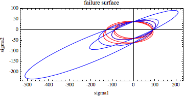
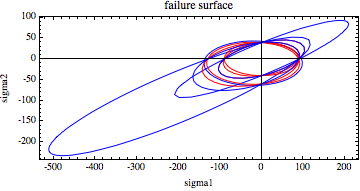
For your second plot, you need the ContourStyle option to style the contours, unsurprisingly enough. You also have several undefined variables, including s45, which I've set to be 50 in the following. There is also a capital S. Please be aware that it is not good practice to name variables with single capital letters as it might clash with a built-in function.
enter image description here

Adding a legend, if that's really what you meant, is quite straightforward in version 9: add the following option to the end of the contour plot and you get the following:

PlotLegends -> Placed[LineLegend[Automatic, 
 {"something", "something else"}], Bottom]
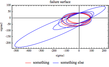
enter image description here

For your second plot, you need the ContourStyle option to style the contours, unsurprisingly enough. You also have several undefined variables, including s45, which I've set to be 50 in the following. There is also a capital S. Please be aware that it is not good practice to name variables with single capital letters as it might clash with a built-in function.

enter image description here

I'm not sure what you mean by it being discontinuous. It doesn't look discontinuous either in a Plot3D or in a Plot holding one variable constant. In fact if you look at the function, at the point that it switches definition, several terms converge to zero no matter which function is being used. So it is actually effectively continuous even if it it isn't continuously differentiable. (It would have helped to remove the Abs[s1c] complication for s1c and s2c and simply used positive variables instead. They don't appear outside Abs expressions.)

For your second plot, you need the ContourStyle option to style the contours, unsurprisingly enough. You also have several undefined variables, including s45, which I've set to be 50 in the following. There is also a capital S. Please be aware that it is not good practice to name variables with single capital letters as it might clash with a built-in function.

enter image description here

Adding a legend, if that's really what you meant, is quite straightforward in version 9: add the following option to the end of the contour plot and you get the following:

PlotLegends -> Placed[LineLegend[Automatic, 
 {"something", "something else"}], Bottom]

enter image description here

added some additional material to cover some side issues
Source Link
Verbeia
  • 34.5k
  • 10
  • 110
  • 225

If you additionally provide a value for S (I used $2$ for the purposes of the next plot), you'll get more contours.

enter image description here

As a side note, the PlotLabel should be a string in quote marks. You only got away with it in this case because multiplying failure and surface results in failure surface in canonical (alphabetical) order.

Source Link
Verbeia
  • 34.5k
  • 10
  • 110
  • 225

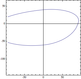
Two issues here: first, as cormullion pointed out in comments, you need the argument of the first ContourPlot to be f[x,y]==1, not just f==1. The reason is that the x and y in your function defition for f are just placeholders, that can substitute for whatever arguments are passed. Mathematica doesn't assume that the x you used in the function definition is the same as the x used in a plot range. So:

ContourPlot[f[x, y] == 1, {x, -30 Pi, 30 Pi}, {y, -45 Pi, 20 Pi}, 
 Axes -> {True, True}]

enter image description here

For your second plot, you need the ContourStyle option to style the contours, unsurprisingly enough. You also have several undefined variables, including s45, which I've set to be 50 in the following. There is also a capital S. Please be aware that it is not good practice to name variables with single capital letters as it might clash with a built-in function.

Having defined s45, the following works:

ContourPlot[{(x/s1t)^2 - x*y/(s1t*s2t) + (y/s2t)^2 == 
   1, (x/s1t)^2 + (y/s2t)^2 + x*y*(1/(s1t^2) - 1/(s2t^2)) == 1, 
  x^2/(s1t^2) + y^2/(s2t^2) - x*y/(s1t^2) == 1, 
  x^2/(s1t*Abs[s1c]) + 
    y^2/(s2t*Abs[s2c]) + (1/s1t - 1/Abs[s1c])*
     x + (1/s2t - 1/Abs[s2c])*y + 
    2*x*y*1/(2*s45^2)*(1 - (1/s1t - 1/Abs[s1c] + 1/s2t - 1/Abs[s2c])*
        s45 - (1/(s1t*Abs[s1c]) + 1/(s2t*Abs[s2c]))*s45^2) == 1, 
  x^2/Abs[(s1t*s1c)] + 
    y^2/Abs[(s2t*s2c)] + (1/s1t - 1/Abs[s1c])*
     x + (1/s2t - 1/Abs[s2c])*y - 1/(2*Sqrt[s1t*s1c*s2t*s2c]) == 1, 
  x^2/Abs[(s1t*s1c)] + 
    y^2/Abs[(s2t*s2c)] + (1/s1t - 1/Abs[s1c])*
     x + (1/s2t - 1/Abs[s2c])*y + 1/Sqrt[s1t*s1c*s2t*s2c] - 
    1/(2*S^2) == 1, (x/s1t)^2 + (y/s2t)^2 == 
   1, (x/s1t)^2 + (y/s2t)^2 - x*y/(s1t*s2t) == 
   1, (x*y - x^2)/(s1t*s1c) - (y^2/(s2t*s2c)) + 
    x*(s1t + s1c)/(s1t*s1c) + y*(s2c + s2t)/(s2t*s2c) == 
   1, (1.95*x*y - x^2)/(s1t*s1c) - (y^2/(s2t*s2c)) + 
    x*(s1c + s1t)/(s1t*s1c) + y*(s2c + s2t)/(s2t*s2c) == 
   1}, {x, -165 Pi, 70 Pi}, {y, -75 Pi, 30 Pi}, Axes -> {True, True}, 
 FrameLabel -> {sigma1, sigma2}, PlotLabel -> "failure surface", 
 AspectRatio -> Automatic, ContourStyle -> {Red, Blue}]

enter image description here