added 1309 characters in body
Source Link
Alex Trounev
  • 48.8k
  • 3
  • 51
  • 115

Figure 3 Figure 4 And finally I give the best result that was obtained in this model with l = 1:

<< NDSolve`FEM`
r = 0.8; ne = 1; kap = 10000; l = 1;
reg = ImplicitRegion[x^2 + y^2 <= 5.3^2, {x, y}];
mesh = ToElementMesh[reg, 
   MeshRefinementFunction -> 
    Function[{vertices, area}, 
     area > 0.0004 (1 + 9 Norm[Mean[vertices]])]];


glass = 1.45; air = 1.; k0 = (2 \[Pi])/1.55; b = I*Sqrt[glass]*k0*1.1;
n[R_] := ( .5*(1 - Tanh[kap*(R - r)])*(glass^2 - air^2) + air^2)*k0^2

helm = -Laplacian[
     u[x, y], {x, y}] - (b^2 + n[Sqrt[x^2 + y^2]] + l^2/(x^2 + y^2))*
    u[x, y];
boundary = DirichletCondition[u[x, y] == 0, True];

{vals, funs} = 
    NDEigensystem[{helm, boundary}, u[x, y], {x, y} \[Element] mesh, 
   ne];


{Show[ mesh["Wireframe"], 
  ContourPlot[x^2 + y^2 == r^2, {x, -1, 1}, {y, -1, 1}, 
   ColorFunction -> Hue]], 
 Show[Plot3D[Im[funs[[1]]], {x, y} \[Element] mesh, PlotRange -> All, 
     PlotLabel -> Row[{"\[Beta] = ", Im[Sqrt[vals[[1]] + b^2]]}], 
   Mesh -> None, ColorFunction -> Hue], 
  Graphics3D[{Gray, Opacity[.4], 
    Cylinder[{{0, 0, -1}, {0, 0, 1.}}, r]}]]}

Figure 5

Figure 3 Figure 4

Figure 3 Figure 4 And finally I give the best result that was obtained in this model with l = 1:

<< NDSolve`FEM`
r = 0.8; ne = 1; kap = 10000; l = 1;
reg = ImplicitRegion[x^2 + y^2 <= 5.3^2, {x, y}];
mesh = ToElementMesh[reg, 
   MeshRefinementFunction -> 
    Function[{vertices, area}, 
     area > 0.0004 (1 + 9 Norm[Mean[vertices]])]];


glass = 1.45; air = 1.; k0 = (2 \[Pi])/1.55; b = I*Sqrt[glass]*k0*1.1;
n[R_] := ( .5*(1 - Tanh[kap*(R - r)])*(glass^2 - air^2) + air^2)*k0^2

helm = -Laplacian[
     u[x, y], {x, y}] - (b^2 + n[Sqrt[x^2 + y^2]] + l^2/(x^2 + y^2))*
    u[x, y];
boundary = DirichletCondition[u[x, y] == 0, True];

{vals, funs} = 
    NDEigensystem[{helm, boundary}, u[x, y], {x, y} \[Element] mesh, 
   ne];


{Show[ mesh["Wireframe"], 
  ContourPlot[x^2 + y^2 == r^2, {x, -1, 1}, {y, -1, 1}, 
   ColorFunction -> Hue]], 
 Show[Plot3D[Im[funs[[1]]], {x, y} \[Element] mesh, PlotRange -> All, 
     PlotLabel -> Row[{"\[Beta] = ", Im[Sqrt[vals[[1]] + b^2]]}], 
   Mesh -> None, ColorFunction -> Hue], 
  Graphics3D[{Gray, Opacity[.4], 
    Cylinder[{{0, 0, -1}, {0, 0, 1.}}, r]}]]}
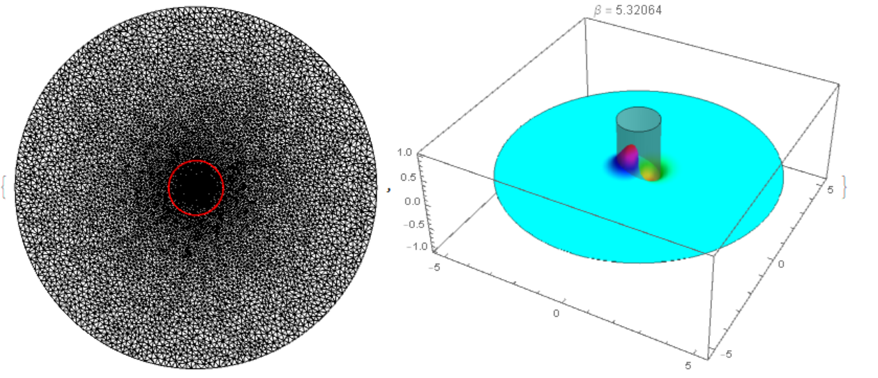
Figure 5

deleted 52 characters in body
Source Link
Alex Trounev
  • 48.8k
  • 3
  • 51
  • 115
<< NDSolve`FEM`
r = 0.8; ne = 10; om = 0.0; kap = 1000; l = 1;
reg = ImplicitRegion[x^2 + y^2 <= 2^2, {x, y}]; f = 
 Function[{vertices, area}, 
  Block[{x, y}, {x, y} = Mean[vertices]; 
   If[x^2 + y^2 <= r^2, area > 0.001, area > 0.01]]];
mesh = ToElementMesh[reg, MeshRefinementFunction -> f];


glass = 1.45; air = 1.; k0 = (2 \[Pi])/1.55; b = I*Sqrt[glass]*k0;
n[R_] := ( .5*(1 - Tanh[kap*(R - r)])*(glass^2 - air^2) + air^2)*k0^2

helm = -Laplacian[
     u[x, y], {x, y}] - (b^2 + n[Sqrt[x^2 + y^2]] + l^2/(x^2 + y^2))*
    u[x, y] + I*om*(x*D[u[x, y], y] - y*D[u[x, y], x]);y];
boundary = DirichletCondition[u[x, y] == 0, True];

{vals, funs} = 
    NDEigensystem[{helm, boundary}, u[x, y], {x, y} \[Element] mesh, 
   ne];

Sqrt[vals + b^2]


(*{0. + 4.93777 I, 0. + 5.29335 I, 0. + 5.29463 I, 
 0. + 3.9743 I, 0. + 3.97351 I, 0. + 3.51044 I, 0. + 3.50924 I, 
 0. + 3.23389 I, 0. + 2.86891 I, 0. + 2.86774 I}*)
{Show[ mesh["Wireframe"], 
  ContourPlot[x^2 + y^2 == r^2, {x, -1, 1}, {y, -1, 1}, 
   ColorFunction -> Hue]], 
 Show[Plot3D[Im[funs[[3]]], {x, y} \[Element] mesh, PlotRange -> All, 
     PlotLabel -> Row[{"\[Beta] = ", Im[Sqrt[vals[[3]] + b^2]]}], 
   Mesh -> None, ColorFunction -> Hue], 
  Graphics3D[{Gray, Opacity[.4], 
    Cylinder[{{0, 0, -1}, {0, 0, 1.}}, r]}]]}

Table[Plot3D[Im[funs[[i]]], {x, y} \[Element] mesh, PlotRange -> All, 
    PlotLabel -> Sqrt[vals[[i]] + b^2], Mesh -> None, 
  ColorFunction -> Hue], {i, Length[vals]}]
<< NDSolve`FEM`
r = 0.8; ne = 10; om = 0.0; kap = 1000; l = 1;
reg = ImplicitRegion[x^2 + y^2 <= 2^2, {x, y}]; f = 
 Function[{vertices, area}, 
  Block[{x, y}, {x, y} = Mean[vertices]; 
   If[x^2 + y^2 <= r^2, area > 0.001, area > 0.01]]];
mesh = ToElementMesh[reg, MeshRefinementFunction -> f];


glass = 1.45; air = 1.; k0 = (2 \[Pi])/1.55; b = I*Sqrt[glass]*k0;
n[R_] := ( .5*(1 - Tanh[kap*(R - r)])*(glass^2 - air^2) + air^2)*k0^2

helm = -Laplacian[
     u[x, y], {x, y}] - (b^2 + n[Sqrt[x^2 + y^2]] + l^2/(x^2 + y^2))*
    u[x, y] + I*om*(x*D[u[x, y], y] - y*D[u[x, y], x]);
boundary = DirichletCondition[u[x, y] == 0, True];

{vals, funs} = 
    NDEigensystem[{helm, boundary}, u[x, y], {x, y} \[Element] mesh, 
   ne];

Sqrt[vals + b^2]


(*{0. + 4.93777 I, 0. + 5.29335 I, 0. + 5.29463 I, 
 0. + 3.9743 I, 0. + 3.97351 I, 0. + 3.51044 I, 0. + 3.50924 I, 
 0. + 3.23389 I, 0. + 2.86891 I, 0. + 2.86774 I}*)
{Show[ mesh["Wireframe"], 
  ContourPlot[x^2 + y^2 == r^2, {x, -1, 1}, {y, -1, 1}, 
   ColorFunction -> Hue]], 
 Show[Plot3D[Im[funs[[3]]], {x, y} \[Element] mesh, PlotRange -> All, 
     PlotLabel -> Row[{"\[Beta] = ", Im[Sqrt[vals[[3]] + b^2]]}], 
   Mesh -> None, ColorFunction -> Hue], 
  Graphics3D[{Gray, Opacity[.4], 
    Cylinder[{{0, 0, -1}, {0, 0, 1.}}, r]}]]}

Table[Plot3D[Im[funs[[i]]], {x, y} \[Element] mesh, PlotRange -> All, 
    PlotLabel -> Sqrt[vals[[i]] + b^2], Mesh -> None, 
  ColorFunction -> Hue], {i, Length[vals]}]
<< NDSolve`FEM`
r = 0.8; ne = 10;  kap = 1000; l = 1;
reg = ImplicitRegion[x^2 + y^2 <= 2^2, {x, y}]; f = 
 Function[{vertices, area}, 
  Block[{x, y}, {x, y} = Mean[vertices]; 
   If[x^2 + y^2 <= r^2, area > 0.001, area > 0.01]]];
mesh = ToElementMesh[reg, MeshRefinementFunction -> f];


glass = 1.45; air = 1.; k0 = (2 \[Pi])/1.55; b = I*Sqrt[glass]*k0;
n[R_] := ( .5*(1 - Tanh[kap*(R - r)])*(glass^2 - air^2) + air^2)*k0^2

helm = -Laplacian[
     u[x, y], {x, y}] - (b^2 + n[Sqrt[x^2 + y^2]] + l^2/(x^2 + y^2))*
    u[x, y];
boundary = DirichletCondition[u[x, y] == 0, True];

{vals, funs} = 
    NDEigensystem[{helm, boundary}, u[x, y], {x, y} \[Element] mesh, 
   ne];

Sqrt[vals + b^2]


(*{0. + 4.93777 I, 0. + 5.29335 I, 0. + 5.29463 I, 
 0. + 3.9743 I, 0. + 3.97351 I, 0. + 3.51044 I, 0. + 3.50924 I, 
 0. + 3.23389 I, 0. + 2.86891 I, 0. + 2.86774 I}*)
{Show[ mesh["Wireframe"], 
  ContourPlot[x^2 + y^2 == r^2, {x, -1, 1}, {y, -1, 1}, 
   ColorFunction -> Hue]], 
 Show[Plot3D[Im[funs[[3]]], {x, y} \[Element] mesh, PlotRange -> All, 
     PlotLabel -> Row[{"\[Beta] = ", Im[Sqrt[vals[[3]] + b^2]]}], 
   Mesh -> None, ColorFunction -> Hue], 
  Graphics3D[{Gray, Opacity[.4], 
    Cylinder[{{0, 0, -1}, {0, 0, 1.}}, r]}]]}

Table[Plot3D[Im[funs[[i]]], {x, y} \[Element] mesh, PlotRange -> All, 
    PlotLabel -> Sqrt[vals[[i]] + b^2], Mesh -> None, 
  ColorFunction -> Hue], {i, Length[vals]}]
added 2257 characters in body
Source Link
Alex Trounev
  • 48.8k
  • 3
  • 51
  • 115

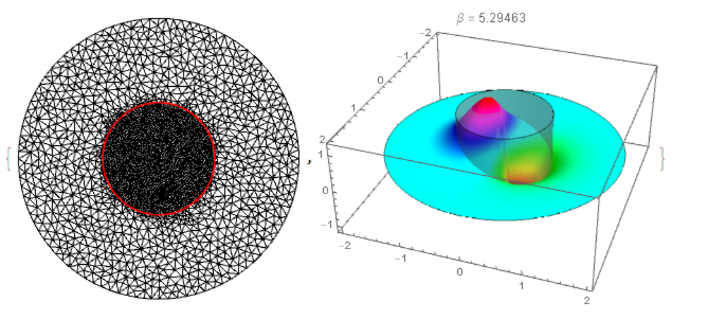
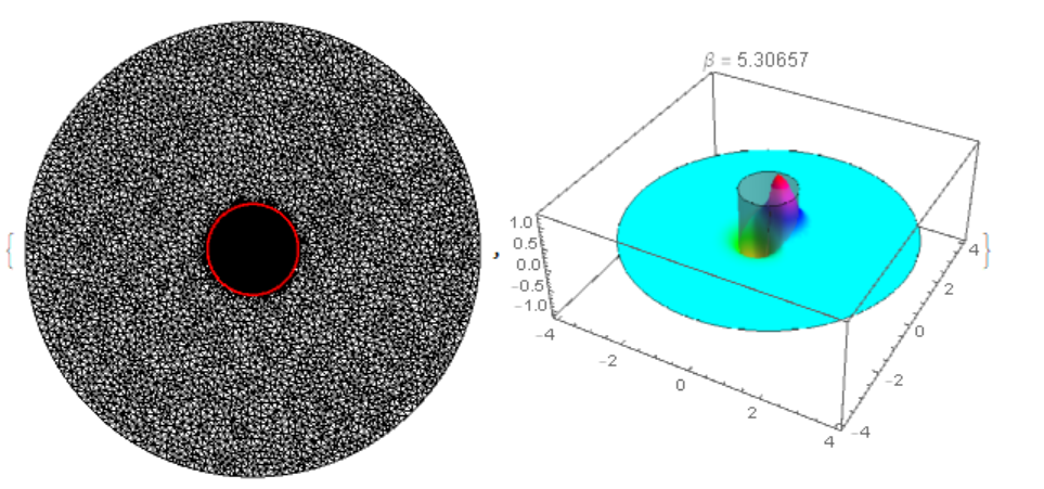
To isolate monotone solutions in the clad with l = 1, we add to the Helmholtz operator (b^2 + l^2/(x^2 + y^2))*u[x, y] and choose eigenfunctions that fade out in the outer region what is achieved when b = I*Sqrt[glass]*k0. Figure 3 shows one of the eigenfunctions. In this case, the desired value $\beta = 5.336$ is achieved with increasing size of the clad. In fig. 4 shows the same eigenfunction with a 2-fold increase in the size of the region of integration.

<< NDSolve`FEM`
r = 0.8; ne = 10; om = 0.0; kap = 1000; l = 1;
reg = ImplicitRegion[x^2 + y^2 <= 2^2, {x, y}]; f = 
 Function[{vertices, area}, 
  Block[{x, y}, {x, y} = Mean[vertices]; 
   If[x^2 + y^2 <= r^2, area > 0.001, area > 0.01]]];
mesh = ToElementMesh[reg, MeshRefinementFunction -> f];


glass = 1.45; air = 1.; k0 = (2 \[Pi])/1.55; b = I*Sqrt[glass]*k0;
n[R_] := ( .5*(1 - Tanh[kap*(R - r)])*(glass^2 - air^2) + air^2)*k0^2

helm = -Laplacian[
     u[x, y], {x, y}] - (b^2 + n[Sqrt[x^2 + y^2]] + l^2/(x^2 + y^2))*
    u[x, y] + I*om*(x*D[u[x, y], y] - y*D[u[x, y], x]);
boundary = DirichletCondition[u[x, y] == 0, True];

{vals, funs} = 
    NDEigensystem[{helm, boundary}, u[x, y], {x, y} \[Element] mesh, 
   ne];

Sqrt[vals + b^2]


(*{0. + 4.93777 I, 0. + 5.29335 I, 0. + 5.29463 I, 
 0. + 3.9743 I, 0. + 3.97351 I, 0. + 3.51044 I, 0. + 3.50924 I, 
 0. + 3.23389 I, 0. + 2.86891 I, 0. + 2.86774 I}*)
{Show[ mesh["Wireframe"], 
  ContourPlot[x^2 + y^2 == r^2, {x, -1, 1}, {y, -1, 1}, 
   ColorFunction -> Hue]], 
 Show[Plot3D[Im[funs[[3]]], {x, y} \[Element] mesh, PlotRange -> All, 
     PlotLabel -> Row[{"\[Beta] = ", Im[Sqrt[vals[[3]] + b^2]]}], 
   Mesh -> None, ColorFunction -> Hue], 
  Graphics3D[{Gray, Opacity[.4], 
    Cylinder[{{0, 0, -1}, {0, 0, 1.}}, r]}]]}

Table[Plot3D[Im[funs[[i]]], {x, y} \[Element] mesh, PlotRange -> All, 
    PlotLabel -> Sqrt[vals[[i]] + b^2], Mesh -> None, 
  ColorFunction -> Hue], {i, Length[vals]}]

Figure 3 Figure 4

added 70 characters in body
Source Link
Alex Trounev
  • 48.8k
  • 3
  • 51
  • 115
Loading
Source Link
Alex Trounev
  • 48.8k
  • 3
  • 51
  • 115
Loading