added 203 characters in body
Source Link
Roman
  • 50k
  • 2
  • 57
  • 132
n = 10;
X = 4N[4/(3*Sqrt[n]3 Sqrt[n])*]*
  SparseArray[{{1,1} -> 1.,
               {-1,-1} -> 1.,
               Band[{2,2}, {-2,-2}] -> 2.,
               Band[{i_2,1}, {-1,1}, {1,0}] ->
                 N@Table[(i-2)^(3/2) - (i-1)^(3/2) + 3+3/2*(i-1)^(1/2), {i,2,n+1}],
               Band[{i_1,-1}, {-2,-1}, {1,0}] -> N@Reverse@Table[(n-i-2)^(3/2) - (ni-i+11)^(3/2) + 3+3/2*(ni-i+11)^(1/2), {i,2,n+1}],
               Sequence @@ Table[Band[{i_1,j_a} /; i !=, j{1+n-a,n}] -> N[a^(3/2)-2*(a-1)^(3/2)+(a-2)^(3/2)], {a,2,n}],
               Sequence @@ (Abs[iTable[Band[{a+1,2}, {n+1,n+2-j]+1)^a}] -> N[a^(3/2) - 2*2(Abs[ia-j]1)^(3/2) + (Abs[i-j]a-12)^(3/2)], {a,2,n}]},
              {n+1, n+1}] // Normal // NNormal;
n = 10;
X = 4/(3*Sqrt[n])*
  SparseArray[{{1,1} -> 1,
               {-1,-1} -> 1,
               Band[{2,2}, {-2,-2}] -> 2,
               {i_,1} -> (i-2)^(3/2) - (i-1)^(3/2) + 3/2*(i-1)^(1/2),
               {i_,-1} -> (n-i)^(3/2) - (n-i+1)^(3/2) + 3/2*(n-i+1)^(1/2),
               {i_,j_} /; i != j ->
                 (Abs[i-j]+1)^(3/2) - 2*(Abs[i-j])^(3/2) + (Abs[i-j]-1)^(3/2)},
              {n+1, n+1}] // Normal // N
n = 10;
X = N[4/(3 Sqrt[n])]*
  SparseArray[{{1,1} -> 1.,
               {-1,-1} -> 1.,
               Band[{2,2}, {-2,-2}] -> 2.,
               Band[{2,1}, {-1,1}, {1,0}] ->
                 N@Table[(i-2)^(3/2)-(i-1)^(3/2)+3/2*(i-1)^(1/2), {i,2,n+1}],
               Band[{1,-1}, {-2,-1}, {1,0}] -> N@Reverse@Table[(i-2)^(3/2)-(i-1)^(3/2)+3/2*(i-1)^(1/2), {i,2,n+1}],
               Sequence @@ Table[Band[{1,a}, {1+n-a,n}] -> N[a^(3/2)-2*(a-1)^(3/2)+(a-2)^(3/2)], {a,2,n}],
               Sequence @@ Table[Band[{a+1,2}, {n+1,n+2-a}] -> N[a^(3/2)-2(a-1)^(3/2)+(a-2)^(3/2)], {a,2,n}]},
              {n+1, n+1}] // Normal;
speedup
Source Link
Roman
  • 50k
  • 2
  • 57
  • 132

Update: much faster version

To speed up this algorithm, the main point is to speed up the calculation of the uintvalues from the uvalues. Instead of doing piecewise integrals, this calculation can be expressed as a matrix multiplication, uintvalues == X.uvalues, with the matrix X defined as

n = 10;
X = 4/(3*Sqrt[n])*
  SparseArray[{{1,1} -> 1,
               {-1,-1} -> 1,
               Band[{2,2}, {-2,-2}] -> 2,
               {i_,1} -> (i-2)^(3/2) - (i-1)^(3/2) + 3/2*(i-1)^(1/2),
               {i_,-1} -> (n-i)^(3/2) - (n-i+1)^(3/2) + 3/2*(n-i+1)^(1/2),
               {i_,j_} /; i != j ->
                 (Abs[i-j]+1)^(3/2) - 2*(Abs[i-j])^(3/2) + (Abs[i-j]-1)^(3/2)},
              {n+1, n+1}] // Normal // N

(The coefficients follow from the Piecewise ansatz and analytic integration.)

With this matrix defined, the algorithm becomes simply

tvalues = Subdivide[n];
f[t_] = 1/3 (-2 Sqrt[1 - t] + 3 t - 4 Sqrt[1 - t] t - 4 t^(3/2));
fvalues = f /@ tvalues;
solution = Inverse[IdentityMatrix[n+1] - X].fvalues
ListLinePlot[Transpose[{tvalues, solution}]]

In this way, $n=1000$ grid points can be achieved in a few seconds, most of which is still spent in assembling the X-matrix. The next step would be to write down a faster way of assembling X.

added 145 characters in body
Source Link
Roman
  • 50k
  • 2
  • 57
  • 132

Here's a general solution that works by interpolation. I'll present the method in a very slow way, and we can work on speeding it up later on if desired.

First, we make an ansatz for the function $u(t)$ on the interval $[0,1]$. Here I use a grid of $n+1$ equidistant points and a linear interpolation scheme:

n = 10;
tvalues = Subdivide[n];
uvalues = Unique[] & /@ tvalues;  (* we don't care what these variables are called *)
tupairs = Transpose[{tvalues, uvalues}];
u[t_] = Piecewise@BlockMap[{((t-#[[2,1]])#[[1,2]]-(t-#[[1,1]])#[[2,2]])/(#[[1, 1]]-#[[2, 1]]),
          #[[1,1]]<=t<=#[[2,1]]}&, tupairs, 2, 1]

Check that this interpolation scheme has indeed the values uvalues on the grid points tvalues:

u /@ tvalues == uvalues
(* True *)

Define the integral $\int_0^1 ds\,u(s)/\sqrt{\lvert t-s\rvert}$:

uint[t_] := Integrate[u[s]/Sqrt[Abs[t-s]], {s, 0, 1}]

Evaluate this integral on the same grid of tvalues: here is the slow part of this calculation, and could probably be sped up dramatically,

uintvalues = uint /@ tvalues
(* long output where every element is a linear combination of the uvalues *)

The right-hand side of the integral equation, evaluated on the same grid of tvalues:

f[t_] = 1/3 (-2 Sqrt[1 - t] + 3 t - 4 Sqrt[1 - t] t - 4 t^(3/2));
fvalues = f /@ tvalues
(* long output *)

Solve for the coefficients of $u(t)$: a linear system of equations for the grid values uvalues, found by setting the left and right sides of the integral equation equal at every grid point in tvalues,

solution = tupairs /.
  First@Solve[Thread[uvalues - uintvalues == fvalues] // N, uvalues]

{{0, 5.84947*10^-16}, {1/10, 0.1}, {1/5, 0.2}, {3/10, 0.3}, {2/5, 0.4}, {1/2, 0.5}, {3/5, 0.6}, {7/10, 0.7}, {4/5, 0.8}, {9/10, 0.9}, {1, 1.}}

This confirms your analytic solution $u(t)=t$ but is much more general.

You don't need the // N in the last step if you prefer an analytic solution; however, numerical solution is very much faster.

ListLinePlot[solution, PlotMarkers -> Automatic]
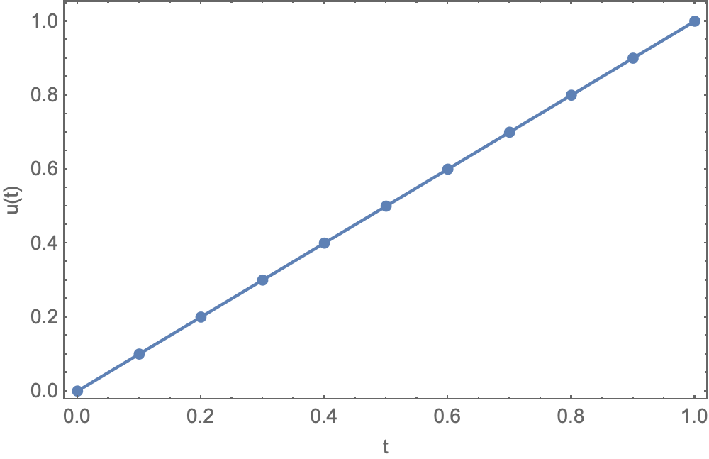
enter image description here

Here's a general solution that works by interpolation. I'll present the method in a very slow way, and we can work on speeding it up later on if desired.

First, we make an ansatz for the function $u(t)$ on the interval $[0,1]$. Here I use a grid of $n+1$ equidistant points and a linear interpolation scheme:

n = 10;
tvalues = Subdivide[n];
uvalues = Unique[] & /@ tvalues;
tupairs = Transpose[{tvalues, uvalues}];
u[t_] = Piecewise@BlockMap[{((t-#[[2,1]])#[[1,2]]-(t-#[[1,1]])#[[2,2]])/(#[[1, 1]]-#[[2, 1]]),
          #[[1,1]]<=t<=#[[2,1]]}&, tupairs, 2, 1]

Check that this interpolation scheme has indeed the values uvalues on the grid points tvalues:

u /@ tvalues == uvalues
(* True *)

Define the integral $\int_0^1 ds\,u(s)/\sqrt{\lvert t-s\rvert}$:

uint[t_] := Integrate[u[s]/Sqrt[Abs[t-s]], {s, 0, 1}]

Evaluate this integral on the same grid of tvalues: here is the slow part of this calculation, and could probably be sped up dramatically,

uintvalues = uint /@ tvalues
(* long output where every element is a linear combination of the uvalues *)

The right-hand side of the integral equation, evaluated on the same grid of tvalues:

f[t_] = 1/3 (-2 Sqrt[1 - t] + 3 t - 4 Sqrt[1 - t] t - 4 t^(3/2));
fvalues = f /@ tvalues
(* long output *)

Solve for the coefficients of $u(t)$: a linear system of equations for the grid values uvalues, found by setting the left and right sides of the integral equation equal at every grid point in tvalues,

solution = tupairs /.
  First@Solve[Thread[uvalues - uintvalues == fvalues] // N, uvalues]

{{0, 5.84947*10^-16}, {1/10, 0.1}, {1/5, 0.2}, {3/10, 0.3}, {2/5, 0.4}, {1/2, 0.5}, {3/5, 0.6}, {7/10, 0.7}, {4/5, 0.8}, {9/10, 0.9}, {1, 1.}}

This confirms your analytic solution $u(t)=t$ but is much more general.

You don't need the // N in the last step if you prefer an analytic solution; however, numerical solution is very much faster.

Here's a general solution that works by interpolation. I'll present the method in a very slow way, and we can work on speeding it up later on if desired.

First, we make an ansatz for the function $u(t)$ on the interval $[0,1]$. Here I use a grid of $n+1$ equidistant points and a linear interpolation scheme:

n = 10;
tvalues = Subdivide[n];
uvalues = Unique[] & /@ tvalues;  (* we don't care what these variables are called *)
tupairs = Transpose[{tvalues, uvalues}];
u[t_] = Piecewise@BlockMap[{((t-#[[2,1]])#[[1,2]]-(t-#[[1,1]])#[[2,2]])/(#[[1, 1]]-#[[2, 1]]),
          #[[1,1]]<=t<=#[[2,1]]}&, tupairs, 2, 1]

Check that this interpolation scheme has indeed the values uvalues on the grid points tvalues:

u /@ tvalues == uvalues
(* True *)

Define the integral $\int_0^1 ds\,u(s)/\sqrt{\lvert t-s\rvert}$:

uint[t_] := Integrate[u[s]/Sqrt[Abs[t-s]], {s, 0, 1}]

Evaluate this integral on the same grid of tvalues: here is the slow part of this calculation, and could probably be sped up dramatically,

uintvalues = uint /@ tvalues
(* long output where every element is a linear combination of the uvalues *)

The right-hand side of the integral equation, evaluated on the same grid of tvalues:

f[t_] = 1/3 (-2 Sqrt[1 - t] + 3 t - 4 Sqrt[1 - t] t - 4 t^(3/2));
fvalues = f /@ tvalues
(* long output *)

Solve for the coefficients of $u(t)$: a linear system of equations for the grid values uvalues, found by setting the left and right sides of the integral equation equal at every grid point in tvalues,

solution = tupairs /.
  First@Solve[Thread[uvalues - uintvalues == fvalues] // N, uvalues]

{{0, 5.84947*10^-16}, {1/10, 0.1}, {1/5, 0.2}, {3/10, 0.3}, {2/5, 0.4}, {1/2, 0.5}, {3/5, 0.6}, {7/10, 0.7}, {4/5, 0.8}, {9/10, 0.9}, {1, 1.}}

This confirms your analytic solution $u(t)=t$ but is much more general.

You don't need the // N in the last step if you prefer an analytic solution; however, numerical solution is very much faster.

ListLinePlot[solution, PlotMarkers -> Automatic]

enter image description here

Source Link
Roman
  • 50k
  • 2
  • 57
  • 132
Loading