Applied some simplifications to make the code more robust and explained how I estimated some parameters.
Source Link
Tim Laska
  • 16.4k
  • 1
  • 35
  • 58

NowTo estimate a characteristic length scale, you need to adjust$y_{10}$, I used the timescale and sampling. Alsomaximum absolute length of $y_1$ from data1 or

ymax = data1[[All, 1]] // Abs // Max (* 0.538851 *)

For the case provided, you will need to consider a goodwe can scale the initial condition for y1'based on the estimate of $y_{10}$ and $\omega$ as functionshown $$y1'(0)=1\rightarrow y1'(0)=\frac{1}{\omega y_{10}}(Dimensionless)\Rightarrow 0.770102$$

Now, you can think of scalethe dimensionless timescale as the number of revolutions in radians. Here is an example Mathematica code. You will need to rescale the data back to dimensional form after the NDSolve. Also note that I combined $m$ and $C_0$ into characteristic frequency $\omega$.

data2 = Block[{omega = 2*Sqrt[5](2 Sqrt[10] 0.5388506382979702`)/Sqrt[2] , 
     y10 = 0.5388506382979702`, v10 = 1}, 
    Reap[NDSolve[{y1''[t] == -y1[t]^3 + (y2[t] - y1[t])^3, 
       y2''[t] == -y2[t]^3 + (y1[t] - y2[t])^3, y1'[0] 
 == 1/omega, 
     y1'[0] == v10/(omega*y10), y1[0] == 0, y2'[0] == 0, y2[0] == 0, 
        WhenEvent[Mod[t, 4 Sqrt[2] \[Pi]/2 omega]\[Pi]] == 0, 
        Sow[{y1[t], y1'[t]}]]}, {}, {t, 0, 200000*Sqrt[5]/omega5000 (2 Pi)}, 
      MaxSteps -> \[Infinity]]]][[Infinity]]][[-1, 1]];
 
ListPlot[data2ListPlot[data3, ImageSize -> Large, PlotRange -> All, 
 PlotStyle -> PointSize[0.0025]]

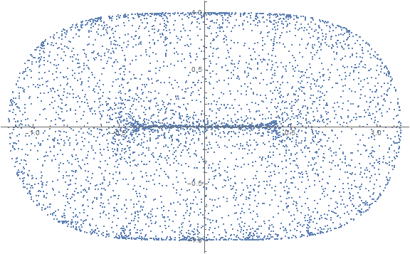
enter image description hereBase case poincare

For molecular vibrations, $\omega$ will be on the order of $10^{13}$$10^{13-14}$ Hz, distances about $0.25x10^{-9}m$, and speed of about $25,000 m/s$ (crude estimates). I also found that I could get a more interesting plot by changingWith the y1' initial condition. Withessentially the followingsame code and just , you can get a result quickly, although I do not claim to know the physical significance. It is more to show that you make NDSolve operate over many orders of magnitude of physical quantities by converting the problem into non-dimensional form.

data3 = Block[{omega = 10^14, 2*Sqrt[5]y10 = 0.25 10^(-9), v10 = 25000}, 
    Reap[NDSolve[{y1''[t] == -y1[t]^3 + (y2[t] - y1[t])^3, 
       y2''[t] == -y2[t]^3 + (y1[t] - y2[t])^3, y1'[0] 
 == omega^(3/2),
     y1'[0] == v10/(omega*y10), y1[0] == 0, y2'[0] == 0, y2[0] == 0, 
        WhenEvent[Mod[t, 4 Sqrt[2] \[Pi]/2 omega]Pi] == 0, 
        Sow[{y1[t], y1'[t]}]]}, {}, {t, 0, 
 200000*Sqrt[5]/omega}, 
      0, 10000 Pi}, MaxSteps -> \[Infinity]]]][[Infinity]]][[-1, 1]];
 

ListPlot[data3, ImageSize -> Large, PlotRange -> All, 
 PlotStyle -> PointSize[0.0025]]

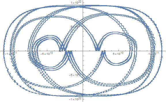
enter image description herePoincare molecular scale

You can note that in data2, that the scaled ymax is indeed one. In the data3 case, they are of order 1 indicating the estimates might be in the right ball park.

Now, you need to adjust the timescale and sampling. Also, you will need to consider a good initial condition for y1' as function of scale. Here is an example Mathematica code. You will need to rescale the data back to dimensional form after the NDSolve. Also note that I combined $m$ and $C_0$ into characteristic frequency $\omega$.

data2 = Block[{omega = 2*Sqrt[5]}, 
    Reap[NDSolve[{y1''[t] == -y1[t]^3 + (y2[t] - y1[t])^3, 
       y2''[t] == -y2[t]^3 + (y1[t] - y2[t])^3, y1'[0] == 1/omega, 
        y1[0] == 0, y2'[0] == 0, y2[0] == 0, 
       WhenEvent[Mod[t, 4 Sqrt[2] \[Pi]/ omega] == 0, 
        Sow[{y1[t], y1'[t]}]]}, {}, {t, 0, 200000*Sqrt[5]/omega}, 
      MaxSteps -> \[Infinity]]]][[-1, 1]];
 
ListPlot[data2, ImageSize -> Large, PlotRange -> All, 
 PlotStyle -> PointSize[0.0025]]

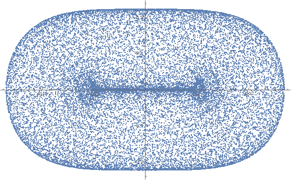
enter image description here

For molecular vibrations, $\omega$ will be on the order of $10^{13}$ Hz. I also found that I could get a more interesting plot by changing the y1' initial condition. With the following code, you can get a result quickly, although I do not claim to know the physical significance. It is more to show that you make NDSolve operate over many orders of magnitude of physical quantities by converting the problem into non-dimensional form.

data3 = Block[{omega = 10^14 2*Sqrt[5]}, 
    Reap[NDSolve[{y1''[t] == -y1[t]^3 + (y2[t] - y1[t])^3, 
       y2''[t] == -y2[t]^3 + (y1[t] - y2[t])^3, y1'[0] == omega^(3/2),
        y1[0] == 0, y2'[0] == 0, y2[0] == 0, 
       WhenEvent[Mod[t, 4 Sqrt[2] \[Pi]/ omega] == 0, 
        Sow[{y1[t], y1'[t]}]]}, {}, {t, 0, 200000*Sqrt[5]/omega}, 
       MaxSteps -> \[Infinity]]]][[-1, 1]];
 

ListPlot[data3, ImageSize -> Large, PlotRange -> All, 
 PlotStyle -> PointSize[0.0025]]

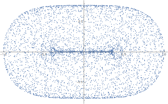
enter image description here

To estimate a characteristic length scale, $y_{10}$, I used the maximum absolute length of $y_1$ from data1 or

ymax = data1[[All, 1]] // Abs // Max (* 0.538851 *)

For the case provided, we can scale the initial condition based on the estimate of $y_{10}$ and $\omega$ as shown $$y1'(0)=1\rightarrow y1'(0)=\frac{1}{\omega y_{10}}(Dimensionless)\Rightarrow 0.770102$$

Now, you can think of the dimensionless timescale as the number of revolutions in radians. Here is an example Mathematica code. You will need to rescale the data back to dimensional form after the NDSolve. Also note that I combined $m$ and $C_0$ into characteristic frequency $\omega$.

data2 = Block[{omega = (2 Sqrt[10] 0.5388506382979702`)/Sqrt[2] , 
     y10 = 0.5388506382979702`, v10 = 1}, 
    Reap[NDSolve[{y1''[t] == -y1[t]^3 + (y2[t] - y1[t])^3, 
       y2''[t] == -y2[t]^3 + (y1[t] - y2[t])^3,  
       y1'[0] == v10/(omega*y10), y1[0] == 0, y2'[0] == 0, y2[0] == 0,
        WhenEvent[Mod[t, 2 \[Pi]] == 0, 
        Sow[{y1[t], y1'[t]}]]}, {}, {t, 0, 5000 (2 Pi)}, 
      MaxSteps -> Infinity]]][[-1, 1]];
ListPlot[data3, ImageSize -> Large, PlotRange -> All, 
 PlotStyle -> PointSize[0.0025]]

Base case poincare

For molecular vibrations, $\omega$ will be on the order of $10^{13-14}$ Hz, distances about $0.25x10^{-9}m$, and speed of about $25,000 m/s$ (crude estimates). With the essentially the same code and just , you can get a result quickly, although I do not claim to know the physical significance. It is more to show that you make NDSolve operate over many orders of magnitude of physical quantities by converting the problem into non-dimensional form.

data3 = Block[{omega = 10^14, y10 = 0.25 10^(-9), v10 = 25000}, 
    Reap[NDSolve[{y1''[t] == -y1[t]^3 + (y2[t] - y1[t])^3, 
       y2''[t] == -y2[t]^3 + (y1[t] - y2[t])^3,  
       y1'[0] == v10/(omega*y10), y1[0] == 0, y2'[0] == 0, y2[0] == 0,
        WhenEvent[Mod[t, 2 Pi] == 0, Sow[{y1[t], y1'[t]}]]}, {}, {t,  
       0, 10000 Pi}, MaxSteps -> Infinity]]][[-1, 1]];

ListPlot[data3, ImageSize -> Large, PlotRange -> All, 
 PlotStyle -> PointSize[0.0025]]

Poincare molecular scale

You can note that in data2, that the scaled ymax is indeed one. In the data3 case, they are of order 1 indicating the estimates might be in the right ball park.
Source Link
Tim Laska
  • 16.4k
  • 1
  • 35
  • 58

If the mass ranges over 25 orders of magnitude, it is likely that other scales, such as the relevant time scale, will also vary over many orders. You can define a characteristic length scale, $y_{10}$ and frequency scale, $\omega = 2{y_{10}}\sqrt {\frac{{{C_0}}}{m}} $ and re-write your equations in dimensionless form. You will have to consider how your initial conditions scale as well.

$$m\frac{{{\partial ^2}y1\left( t \right)}}{{\partial {t^2}}} = 4{C_0}{\left( {y2\left( t \right) - y1\left( t \right)} \right)^3} - 4{C_0}y1{\left( t \right)^3}$$ $$\frac{{{\partial ^2}y2\left( t \right)}}{{\partial {t^2}}} = 4{C_0}{\left( {y1\left( t \right) - y2\left( t \right)} \right)^3} - 4{C_0}y2{\left( t \right)^3}$$

In dimensionless form, they become:

$$\frac{{{\partial ^2}y1\left( t \right)}}{{\partial {t^2}}} = {\left( {y2\left( t \right) - y1\left( t \right)} \right)^3} - y1{\left( t \right)^3}$$ $$\frac{{{\partial ^2}y2\left( t \right)}}{{\partial {t^2}}} = {\left( {y1\left( t \right) - y2\left( t \right)} \right)^3} - y2{\left( t \right)^3}$$

Now, you need to adjust the timescale and sampling. Also, you will need to consider a good initial condition for y1' as function of scale. Here is an example Mathematica code. You will need to rescale the data back to dimensional form after the NDSolve. Also note that I combined $m$ and $C_0$ into characteristic frequency $\omega$.

data2 = Block[{omega = 2*Sqrt[5]}, 
    Reap[NDSolve[{y1''[t] == -y1[t]^3 + (y2[t] - y1[t])^3, 
       y2''[t] == -y2[t]^3 + (y1[t] - y2[t])^3, y1'[0] == 1/omega, 
       y1[0] == 0, y2'[0] == 0, y2[0] == 0, 
       WhenEvent[Mod[t, 4 Sqrt[2] \[Pi]/ omega] == 0, 
        Sow[{y1[t], y1'[t]}]]}, {}, {t, 0, 200000*Sqrt[5]/omega}, 
      MaxSteps -> \[Infinity]]]][[-1, 1]];

ListPlot[data2, ImageSize -> Large, PlotRange -> All, 
 PlotStyle -> PointSize[0.0025]]

enter image description here

For molecular vibrations, $\omega$ will be on the order of $10^{13}$ Hz. I also found that I could get a more interesting plot by changing the y1' initial condition. With the following code, you can get a result quickly, although I do not claim to know the physical significance. It is more to show that you make NDSolve operate over many orders of magnitude of physical quantities by converting the problem into non-dimensional form.

data3 = Block[{omega = 10^14 2*Sqrt[5]}, 
    Reap[NDSolve[{y1''[t] == -y1[t]^3 + (y2[t] - y1[t])^3, 
       y2''[t] == -y2[t]^3 + (y1[t] - y2[t])^3, y1'[0] == omega^(3/2),
        y1[0] == 0, y2'[0] == 0, y2[0] == 0, 
       WhenEvent[Mod[t, 4 Sqrt[2] \[Pi]/ omega] == 0, 
        Sow[{y1[t], y1'[t]}]]}, {}, {t, 0, 200000*Sqrt[5]/omega}, 
      MaxSteps -> \[Infinity]]]][[-1, 1]];


ListPlot[data3, ImageSize -> Large, PlotRange -> All, 
 PlotStyle -> PointSize[0.0025]]

enter image description here