I have an approach that is similar to Hendrik's but is a bit more streamlined and possibly more efficient.
Let's start with some definitions and the mesh:
f = 10*Exp[-(Power[x - 0.5, 2] + Power[y - 0.5, 2])/0.02];
g = -Sin[5*x];

Needs["NDSolve`FEM`"]
mesh = ToElementMesh[Rectangle[]];
Then there is a utility function that is not documented that we can use here. It's purpose to the take a PDE, BCs, ics and a region and generate the discretized versions from them. I'll use the same names, then it should be clear what the function does.
{dpde, dbc, vd, sd, mdata} =
  ProcessPDEEquations[{-Laplacian[u[x, y], {x, y}]
     == f + NeumannValue[g, True]}, u, {x, y} \[Element] mesh];
{load, stiffness, damping, mass} = dpde["All"];
DeployBoundaryConditions[{load, stiffness}, dbc];
This generates the same data as in Hendrik's post. Now, we write a helper function that implements the integral constraint. We need, loosely speaking, the contribution of each node to the total area of the region. Now, there is the mesh["MeshElementMeasure"] which gives the area contribution of each element. What we are looking for is the 'area' contribution 'surrounding' each mesh node, figuratively speaking. Hendrik extracted that information from the mass matrix. I used the load vector. That should be a bit more efficient and needs less data massaging. But it the same principal. To get those values we use the discretization mechanism we already have. We set the load coefficient to 1. If you were to sum some over the discretized load vector, you'd get the area of the region. The constraint matrix contains the value we like this integral to be, 0 in this case. Then I fill in the data structure that DeployBoundaryCondition needs.
FEMIntegralConstraint[value_, methodData_, vd_, sd_] := Module[
  {prec, dof, loadContribution, stiffnessContribution, initCoeffs,
   constraintMatrix, constraintRows, constraintValueMatrix},

  prec = methodData["Precision"];
  dof = methodData["DegreesOfFreedom"];

  (* no values are added to the load vector and stiffness matrix *)
  loadContribution = SparseArray[{}, {dof, 1}, N[0, prec]];
  stiffnessContribution = SparseArray[{}, {dof, dof}, N[0, prec]];

  (* init the load coefficient to 1 *)
  initCoeffs = InitializePDECoefficients[vd, sd, "LoadCoefficients" -> {{1}}];

  (* values inserted into the stiffness matrix overwriting what there was *)
  constraintMatrix = Transpose[
    DiscretizePDE[initCoeffs, methodData, sd]["LoadVector"]];

  constraintRows = {1};
  (* values inseted into the load vector, overwriting what there was *)
    constraintValueMatrix = SparseArray[{{N[value, prec]}}];

  DiscretizedBoundaryConditionData[{loadContribution,
    stiffnessContribution, constraintMatrix, constraintRows,
    constraintValueMatrix,
    (* DOF, hanging nodes DOF,
    lagrangian multipliers DOF *)
    {dof, 0, Length[constraintRows]}},
   (* scale factor value *)
   1]
  ]
With this in place we can now construct the integral constraint and deploy those. "Append" means those constraints are appended to the system matrices (as Lagrange multipliers)
dbc = FEMIntegralConstraint[0, mdata, vd, sd]
DeployBoundaryConditions[{load, stiffness}, dbc,
 "ConstraintMethod" -> "Append" ]
The rest is the same:
v = LinearSolve[stiffness, load];
solfun3 =
  ElementMeshInterpolation[{mesh}, Take[v, mdata["DegreesOfFreedom"]]];
We can check that the constraint worked:
NIntegrate[solfun3[x, y], {x, y} \[Element] mesh]
1.1645204900769326`*^-7
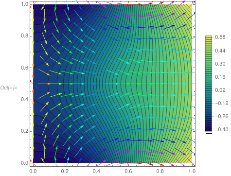
Which is quite acceptable, I think. Also there is no difference to the result Hendrik provided.
Show[ContourPlot[solfun3[x, y], {x, y} \[Element] mesh,
  PlotLegends -> Automatic, Contours -> 50,
  ColorFunction -> "BlueGreenYellow"],
 VectorPlot[
  Evaluate[Grad[solfun3[x, y], {x, y}]], {x, y} \[Element] mesh,
  VectorColorFunction -> Hue, VectorScale -> {Small, 0.6, None}]]

One thing is that the result on your linked page seems to have a bit higher a max value, but I may be wrong. If you have it installed, I'd check the values.

