better explanation
Source Link
Alper91
  • 137
  • 8

I have 2 functions;

funtion 1:

ctr = {(Exp[Pi*0.5] + 1)/2, 0};
radius = (Exp[Pi*0.5] - 1)/2;
pp = PolarPlot[
  Evaluate@Table[Exp[(t + 2*Pi*i/120)*0.5], {i, 1, 120}], {t, -Pi, 
   Pi}, RegionFunction -> (Norm[{#, #2} - ctr] <= radius &)]
Total[ArcLength /@ Cases[pp, _Line, All]]

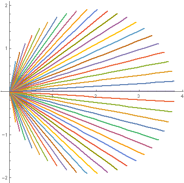
spiral

and function 2:

ctr = {(Exp[Pi*0.5] - 1)/2, 0};
radius = (Exp[Pi*0.5] - 1)/2;
pp2 = ParametricPlot[
  Evaluate[Table[{t, t (Tan[2 j Pi / 120])}, {j, 1, 60}]], {t, -5, 5},
   RegionFunction -> (Norm[{#, #2} - ctr] <= radius &), 
  PlotRange -> All]
Total[ArcLength /@ Cases[pp2, _Line, All]]

Line

I want to show that function 1 is distributed within the circle more homogeneously than function 2 as it is inferred by the graphs. It is clearly seen that function 1 is more homogeneous but I need to support it by the data. How can I show it in mathematica?

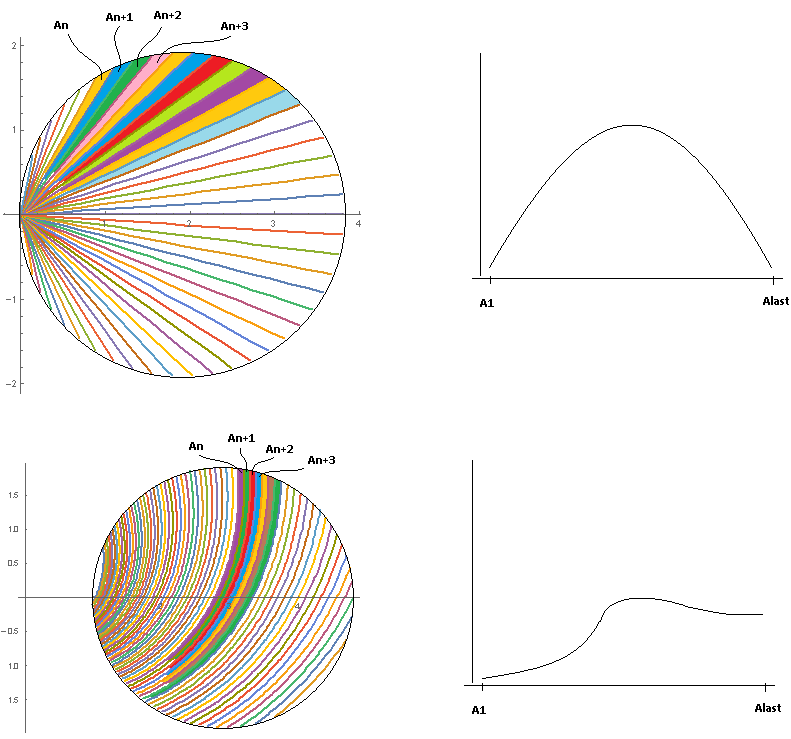
Maybe, the area between the lines in the intersection circle give me what I want as below:

gradient

I can show that the maximum missing spaces between the lines are less in function 1.

I have 2 functions;

funtion 1:

ctr = {(Exp[Pi*0.5] + 1)/2, 0};
radius = (Exp[Pi*0.5] - 1)/2;
pp = PolarPlot[
  Evaluate@Table[Exp[(t + 2*Pi*i/120)*0.5], {i, 1, 120}], {t, -Pi, 
   Pi}, RegionFunction -> (Norm[{#, #2} - ctr] <= radius &)]
Total[ArcLength /@ Cases[pp, _Line, All]]

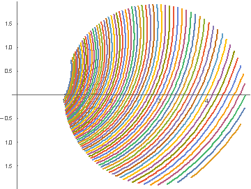
spiral

and function 2:

ctr = {(Exp[Pi*0.5] - 1)/2, 0};
radius = (Exp[Pi*0.5] - 1)/2;
pp2 = ParametricPlot[
  Evaluate[Table[{t, t (Tan[2 j Pi / 120])}, {j, 1, 60}]], {t, -5, 5},
   RegionFunction -> (Norm[{#, #2} - ctr] <= radius &), 
  PlotRange -> All]
Total[ArcLength /@ Cases[pp2, _Line, All]]

Line

I want to show that function 1 is distributed within the circle more homogeneously than function 2 as it is inferred by the graphs. It is clearly seen that function 1 is more homogeneous but I need to support it by the data. How can I show it in mathematica?

Maybe, the area between the lines in the intersection circle give me what I want as below:

gradient

I can show that the maximum missing spaces between the lines are less in function 1.
Source Link
Alper91
  • 137
  • 8

Homogeneity of a function within a region

I have 2 functions;

funtion 1:

ctr = {(Exp[Pi*0.5] + 1)/2, 0};
radius = (Exp[Pi*0.5] - 1)/2;
pp = PolarPlot[
  Evaluate@Table[Exp[(t + 2*Pi*i/120)*0.5], {i, 1, 120}], {t, -Pi, 
   Pi}, RegionFunction -> (Norm[{#, #2} - ctr] <= radius &)]
Total[ArcLength /@ Cases[pp, _Line, All]]

spiral

and function 2:

ctr = {(Exp[Pi*0.5] - 1)/2, 0};
radius = (Exp[Pi*0.5] - 1)/2;
pp2 = ParametricPlot[
  Evaluate[Table[{t, t (Tan[2 j Pi / 120])}, {j, 1, 60}]], {t, -5, 5},
   RegionFunction -> (Norm[{#, #2} - ctr] <= radius &), 
  PlotRange -> All]
Total[ArcLength /@ Cases[pp2, _Line, All]]

Line

I want to show that function 1 is distributed within the circle more homogeneously than function 2 as it is inferred by the graphs. It is clearly seen that function 1 is more homogeneous but I need to support it by the data. How can I show it in mathematica?