Bounty Ended with 100 reputation awarded by user21
added 2 characters in body
Source Link
Henrik Schumacher
  • 109.4k
  • 7
  • 186
  • 322

That's a typical problem; it is caused by the matrix of the discretized system having a one-dimensiondimensional kernel (and cokernel). One can stabilize the system by adding a row and a column that represent a homogeneous mean-value constraint. I don't know whether NDSolve can do that (user21 will be able to tell us), but one can do that with low-level FEM-programming:

Needs["NDSolve`FEM`"]
bmesh = ToBoundaryMesh[
   "Coordinates" -> {{0., 0.}, {1, 0.}, {1, 1}, {0., 1}, {0.5, 0.5}}, 
   "BoundaryElements" -> {LineElement[{{1, 2}, {2, 3}, {3, 4}, {4, 1}}]}];
mesh = ToElementMesh[bmesh, "MaxCellMeasure" -> 0.001];

vd = NDSolve`VariableData[{"DependentVariables", "Space"} -> {{u}, {x, y}}];
sd = NDSolve`SolutionData[{"Space"} -> {mesh}];
cdata = InitializePDECoefficients[vd, sd, 
   "DiffusionCoefficients" -> {{-IdentityMatrix[2]}}, 
   "MassCoefficients" -> {{1}}, 
   "LoadCoefficients" -> {{f}}
   ];
bcdata = InitializeBoundaryConditions[vd, sd, {{NeumannValue[g, True]}}];
mdata = InitializePDEMethodData[vd, sd];

(*Discretization*)
dpde = DiscretizePDE[cdata, mdata, sd];
dbc = DiscretizeBoundaryConditions[bcdata, mdata, sd];
{load, stiffness, damping, mass} = dpde["All"];
mass0 = mass;
DeployBoundaryConditions[{load, stiffness}, dbc];

enter image description here

Here the warning message is created. We ignore it because we augment the stiffness matrix in the following way:

a = SparseArray[{Total[mass0]}];
L = ArrayFlatten[{{stiffness, Transpose[a]}, {a, 0.}}];
b = Flatten[Join[load, {0.}]];
v = LinearSolve[L, b, Method -> "Pardiso"][[1 ;; Length[mass]]];

Now we can plot the solution:

solfun = ElementMeshInterpolation[{mesh}, v];
DensityPlot[solfun[x, y], {x, y} ∈ mesh, 
 ColorFunction -> "SunsetColors"]

enter image description here

I leave the cosmethicscosmetics to you. Beware that the derivativederivatives of these finite-element solutions are guaranteed to be close to the actual solution only in the $L^2$-norm. So it may happen that the gradient vector field looks much rougher than you would expect.

That's a typical problem; it is caused by the matrix of the discretized system having a one-dimension kernel (and cokernel). One can stabilize the system by adding a row and a column that represent a homogeneous mean-value constraint. I don't know whether NDSolve can do that (user21 will be able to tell us), but one can do that with low-level FEM-programming:

Needs["NDSolve`FEM`"]
bmesh = ToBoundaryMesh[
   "Coordinates" -> {{0., 0.}, {1, 0.}, {1, 1}, {0., 1}, {0.5, 0.5}}, 
   "BoundaryElements" -> {LineElement[{{1, 2}, {2, 3}, {3, 4}, {4, 1}}]}];
mesh = ToElementMesh[bmesh, "MaxCellMeasure" -> 0.001];

vd = NDSolve`VariableData[{"DependentVariables", "Space"} -> {{u}, {x, y}}];
sd = NDSolve`SolutionData[{"Space"} -> {mesh}];
cdata = InitializePDECoefficients[vd, sd, 
   "DiffusionCoefficients" -> {{-IdentityMatrix[2]}}, 
   "MassCoefficients" -> {{1}}, 
   "LoadCoefficients" -> {{f}}
   ];
bcdata = InitializeBoundaryConditions[vd, sd, {{NeumannValue[g, True]}}];
mdata = InitializePDEMethodData[vd, sd];

(*Discretization*)
dpde = DiscretizePDE[cdata, mdata, sd];
dbc = DiscretizeBoundaryConditions[bcdata, mdata, sd];
{load, stiffness, damping, mass} = dpde["All"];
mass0 = mass;
DeployBoundaryConditions[{load, stiffness}, dbc];

enter image description here

Here the warning message is created. We ignore it because we augment the stiffness matrix in the following way:

a = SparseArray[{Total[mass0]}];
L = ArrayFlatten[{{stiffness, Transpose[a]}, {a, 0.}}];
b = Flatten[Join[load, {0.}]];
v = LinearSolve[L, b, Method -> "Pardiso"][[1 ;; Length[mass]]];

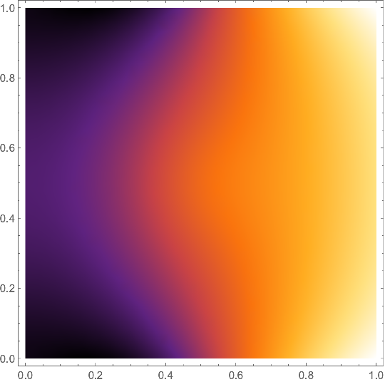
Now we can plot the solution:

solfun = ElementMeshInterpolation[{mesh}, v];
DensityPlot[solfun[x, y], {x, y} ∈ mesh, 
 ColorFunction -> "SunsetColors"]

enter image description here

I leave the cosmethics to you. Beware that the derivative of these finite-element solutions are guaranteed to be close to the actual solution only in the $L^2$-norm. So it may happen that the gradient vector field looks much rougher than you would expect.
That's a typical problem; it is caused by the matrix of the discretized system having a one-dimensional kernel (and cokernel). One can stabilize the system by adding a row and a column that represent a homogeneous mean-value constraint. I don't know whether NDSolve can do that (user21 will be able to tell us), but one can do that with low-level FEM-programming:

Needs["NDSolve`FEM`"]
bmesh = ToBoundaryMesh[
   "Coordinates" -> {{0., 0.}, {1, 0.}, {1, 1}, {0., 1}, {0.5, 0.5}}, 
   "BoundaryElements" -> {LineElement[{{1, 2}, {2, 3}, {3, 4}, {4, 1}}]}];
mesh = ToElementMesh[bmesh, "MaxCellMeasure" -> 0.001];

vd = NDSolve`VariableData[{"DependentVariables", "Space"} -> {{u}, {x, y}}];
sd = NDSolve`SolutionData[{"Space"} -> {mesh}];
cdata = InitializePDECoefficients[vd, sd, 
   "DiffusionCoefficients" -> {{-IdentityMatrix[2]}}, 
   "MassCoefficients" -> {{1}}, 
   "LoadCoefficients" -> {{f}}
   ];
bcdata = InitializeBoundaryConditions[vd, sd, {{NeumannValue[g, True]}}];
mdata = InitializePDEMethodData[vd, sd];

(*Discretization*)
dpde = DiscretizePDE[cdata, mdata, sd];
dbc = DiscretizeBoundaryConditions[bcdata, mdata, sd];
{load, stiffness, damping, mass} = dpde["All"];
mass0 = mass;
DeployBoundaryConditions[{load, stiffness}, dbc];

enter image description here

Here the warning message is created. We ignore it because we augment the stiffness matrix in the following way:

a = SparseArray[{Total[mass0]}];
L = ArrayFlatten[{{stiffness, Transpose[a]}, {a, 0.}}];
b = Flatten[Join[load, {0.}]];
v = LinearSolve[L, b, Method -> "Pardiso"][[1 ;; Length[mass]]];

Now we can plot the solution:

solfun = ElementMeshInterpolation[{mesh}, v];
DensityPlot[solfun[x, y], {x, y} ∈ mesh, 
 ColorFunction -> "SunsetColors"]

enter image description here

I leave the cosmetics to you. Beware that the derivatives of these finite-element solutions are guaranteed to be close to the actual solution only in the $L^2$-norm. So it may happen that the gradient vector field looks much rougher than you would expect.

added 12 characters in body
Source Link
Henrik Schumacher
  • 109.4k
  • 7
  • 186
  • 322

That's a typical problem becauseproblem; it is caused by the matrix of the discretized system hashaving a one-dimension kernel (and cokernel). One can stabilize the system by adding a row and a column that represent a homogeneous mean-value constraint. I don't know whether NDSolve can do that (user21 will be able to tell us), but one can do that with low-level FEM-programming:

Needs["NDSolve`FEM`"]
bmesh = ToBoundaryMesh[
   "Coordinates" -> {{0., 0.}, {1, 0.}, {1, 1}, {0., 1}, {0.5, 0.5}}, 
   "BoundaryElements" -> {LineElement[{{1, 2}, {2, 3}, {3, 4}, {4, 1}}]}];
mesh = ToElementMesh[bmesh, "MaxCellMeasure" -> 0.001];

vd = NDSolve`VariableData[{"DependentVariables", "Space"} -> {{u}, {x, y}}];
sd = NDSolve`SolutionData[{"Space"} -> {mesh}];
cdata = InitializePDECoefficients[vd, sd, 
   "DiffusionCoefficients" -> {{-IdentityMatrix[2]}}, 
   "MassCoefficients" -> {{1}}, 
   "LoadCoefficients" -> {{f}}
   ];
bcdata = InitializeBoundaryConditions[vd, sd, {{NeumannValue[g, True]}}];
mdata = InitializePDEMethodData[vd, sd];

(*Discretization*)
dpde = DiscretizePDE[cdata, mdata, sd];
dbc = DiscretizeBoundaryConditions[bcdata, mdata, sd];
{load, stiffness, damping, mass} = dpde["All"];
mass0 = mass;
DeployBoundaryConditions[{load, stiffness}, dbc];

enter image description here

Here the warning message is created. We ignore it because we augment the stiffness matrix in the following way:

a = SparseArray[{Total[mass0]}];
L = ArrayFlatten[{{stiffness, Transpose[a]}, {a, 0.}}];
b = Flatten[Join[load, {0.}]];
v = LinearSolve[L, b, Method -> "Pardiso"][[1 ;; Length[mass]]];

Now we can plot the solution:

solfun = ElementMeshInterpolation[{mesh}, v];
DensityPlot[solfun[x, y], {x, y} ∈ mesh, 
 ColorFunction -> "SunsetColors"]

enter image description here

I leave the cosmethics to you. Beware that the derivative of these finite-element solutions are guaranteed to be close to the actual solution only in the $L^2$-norm. So it may happen that the gradient vector field looks much rougher than you would expect.

That's a typical problem because the matrix of the discretized system has a one-dimension kernel (and cokernel). One can stabilize the system by adding a row and a column that represent a homogeneous mean-value constraint. I don't know whether NDSolve can do that (user21 will be able to tell us), but one can do that with low-level FEM-programming:

Needs["NDSolve`FEM`"]
bmesh = ToBoundaryMesh[
   "Coordinates" -> {{0., 0.}, {1, 0.}, {1, 1}, {0., 1}, {0.5, 0.5}}, 
   "BoundaryElements" -> {LineElement[{{1, 2}, {2, 3}, {3, 4}, {4, 1}}]}];
mesh = ToElementMesh[bmesh, "MaxCellMeasure" -> 0.001];

vd = NDSolve`VariableData[{"DependentVariables", "Space"} -> {{u}, {x, y}}];
sd = NDSolve`SolutionData[{"Space"} -> {mesh}];
cdata = InitializePDECoefficients[vd, sd, 
   "DiffusionCoefficients" -> {{-IdentityMatrix[2]}}, 
   "MassCoefficients" -> {{1}}, "LoadCoefficients" -> {{f}}];
bcdata = InitializeBoundaryConditions[vd, sd, {{NeumannValue[g, True]}}];
mdata = InitializePDEMethodData[vd, sd];

(*Discretization*)
dpde = DiscretizePDE[cdata, mdata, sd];
dbc = DiscretizeBoundaryConditions[bcdata, mdata, sd];
{load, stiffness, damping, mass} = dpde["All"];
mass0 = mass;
DeployBoundaryConditions[{load, stiffness}, dbc];

enter image description here

Here the warning message is created. We ignore it because we augment the stiffness matrix in the following way:

a = SparseArray[{Total[mass0]}];
L = ArrayFlatten[{{stiffness, Transpose[a]}, {a, 0.}}];
b = Flatten[Join[load, {0.}]];
v = LinearSolve[L, b, Method -> "Pardiso"][[1 ;; Length[mass]]];

Now we can plot the solution:

solfun = ElementMeshInterpolation[{mesh}, v];
DensityPlot[solfun[x, y], {x, y} ∈ mesh, 
 ColorFunction -> "SunsetColors"]

enter image description here

I leave the cosmethics to you. Beware that the derivative of these finite-element solutions are guaranteed to be close to the actual solution only in the $L^2$-norm. So it may happen that the gradient vector field looks much rougher than you would expect.

That's a typical problem; it is caused by the matrix of the discretized system having a one-dimension kernel (and cokernel). One can stabilize the system by adding a row and a column that represent a homogeneous mean-value constraint. I don't know whether NDSolve can do that (user21 will be able to tell us), but one can do that with low-level FEM-programming:

Needs["NDSolve`FEM`"]
bmesh = ToBoundaryMesh[
   "Coordinates" -> {{0., 0.}, {1, 0.}, {1, 1}, {0., 1}, {0.5, 0.5}}, 
   "BoundaryElements" -> {LineElement[{{1, 2}, {2, 3}, {3, 4}, {4, 1}}]}];
mesh = ToElementMesh[bmesh, "MaxCellMeasure" -> 0.001];

vd = NDSolve`VariableData[{"DependentVariables", "Space"} -> {{u}, {x, y}}];
sd = NDSolve`SolutionData[{"Space"} -> {mesh}];
cdata = InitializePDECoefficients[vd, sd, 
   "DiffusionCoefficients" -> {{-IdentityMatrix[2]}}, 
   "MassCoefficients" -> {{1}}, 
   "LoadCoefficients" -> {{f}}
   ];
bcdata = InitializeBoundaryConditions[vd, sd, {{NeumannValue[g, True]}}];
mdata = InitializePDEMethodData[vd, sd];

(*Discretization*)
dpde = DiscretizePDE[cdata, mdata, sd];
dbc = DiscretizeBoundaryConditions[bcdata, mdata, sd];
{load, stiffness, damping, mass} = dpde["All"];
mass0 = mass;
DeployBoundaryConditions[{load, stiffness}, dbc];

enter image description here

Here the warning message is created. We ignore it because we augment the stiffness matrix in the following way:

a = SparseArray[{Total[mass0]}];
L = ArrayFlatten[{{stiffness, Transpose[a]}, {a, 0.}}];
b = Flatten[Join[load, {0.}]];
v = LinearSolve[L, b, Method -> "Pardiso"][[1 ;; Length[mass]]];

Now we can plot the solution:

solfun = ElementMeshInterpolation[{mesh}, v];
DensityPlot[solfun[x, y], {x, y} ∈ mesh, 
 ColorFunction -> "SunsetColors"]

enter image description here

I leave the cosmethics to you. Beware that the derivative of these finite-element solutions are guaranteed to be close to the actual solution only in the $L^2$-norm. So it may happen that the gradient vector field looks much rougher than you would expect.

Source Link
Henrik Schumacher
  • 109.4k
  • 7
  • 186
  • 322

That's a typical problem because the matrix of the discretized system has a one-dimension kernel (and cokernel). One can stabilize the system by adding a row and a column that represent a homogeneous mean-value constraint. I don't know whether NDSolve can do that (user21 will be able to tell us), but one can do that with low-level FEM-programming:

Needs["NDSolve`FEM`"]
bmesh = ToBoundaryMesh[
   "Coordinates" -> {{0., 0.}, {1, 0.}, {1, 1}, {0., 1}, {0.5, 0.5}}, 
   "BoundaryElements" -> {LineElement[{{1, 2}, {2, 3}, {3, 4}, {4, 1}}]}];
mesh = ToElementMesh[bmesh, "MaxCellMeasure" -> 0.001];

vd = NDSolve`VariableData[{"DependentVariables", "Space"} -> {{u}, {x, y}}];
sd = NDSolve`SolutionData[{"Space"} -> {mesh}];
cdata = InitializePDECoefficients[vd, sd, 
   "DiffusionCoefficients" -> {{-IdentityMatrix[2]}}, 
   "MassCoefficients" -> {{1}}, "LoadCoefficients" -> {{f}}];
bcdata = InitializeBoundaryConditions[vd, sd, {{NeumannValue[g, True]}}];
mdata = InitializePDEMethodData[vd, sd];

(*Discretization*)
dpde = DiscretizePDE[cdata, mdata, sd];
dbc = DiscretizeBoundaryConditions[bcdata, mdata, sd];
{load, stiffness, damping, mass} = dpde["All"];
mass0 = mass;
DeployBoundaryConditions[{load, stiffness}, dbc];

enter image description here

Here the warning message is created. We ignore it because we augment the stiffness matrix in the following way:

a = SparseArray[{Total[mass0]}];
L = ArrayFlatten[{{stiffness, Transpose[a]}, {a, 0.}}];
b = Flatten[Join[load, {0.}]];
v = LinearSolve[L, b, Method -> "Pardiso"][[1 ;; Length[mass]]];

Now we can plot the solution:

solfun = ElementMeshInterpolation[{mesh}, v];
DensityPlot[solfun[x, y], {x, y} ∈ mesh, 
 ColorFunction -> "SunsetColors"]

enter image description here

I leave the cosmethics to you. Beware that the derivative of these finite-element solutions are guaranteed to be close to the actual solution only in the $L^2$-norm. So it may happen that the gradient vector field looks much rougher than you would expect.