added 1254 characters in body
Source Link
Alex Trounev
  • 48.8k
  • 3
  • 51
  • 115

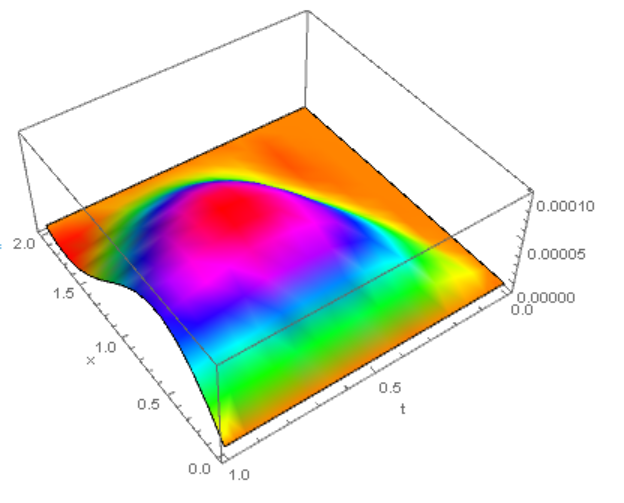
Numerical solution visualization Figure 2
Now we will check how many points are used or this solution:

Needs["DifferentialEquations`InterpolatingFunctionAnatomy`"];

Map[Length, InterpolatingFunctionCoordinates[sol1]]

Out[]= {100, 26}

These 26 points are not enough to find the frequencies, so we will add an option to increase the number of points

AbsoluteTiming[
 sol2 = NDSolveValue[{D[Elastic*Imoment*D[w[x, t], {x, 2}], {x, 2}] + 
       S*rho*D[w[x, t], {t, 2}] - Fnu[x, t] == 0, 
     w[0, t] == w[L, t] == w[x, 0] == 0, 
     Derivative[2, 0][w][0, t] == Derivative[2, 0][w][L, t] == 
      Derivative[0, 1][w][x, 0] == 0}, w, {x, 0, L}, {t, 0, tau}, 
    Method -> {"MethodOfLines", 
      "DifferentiateBoundaryConditions" -> False, 
      "SpatialDiscretization" -> {"TensorProductGrid", 
        "MaxPoints" -> 100, "MinPoints" -> 100, 
        "DifferenceOrder" -> 2}}, MaxStepSize -> 0.05, 
    EvaluationMonitor :> (currentTime = t;)];]

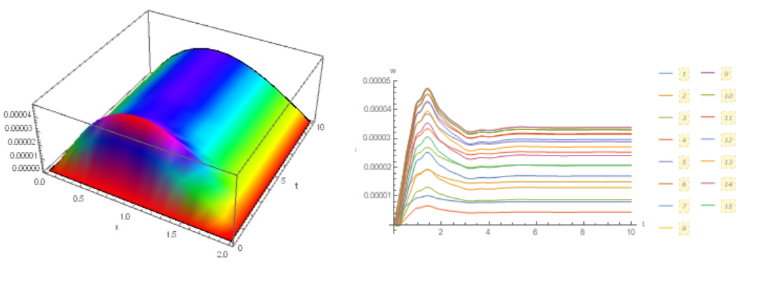
Here we see a periodic solution with a period of 2.5: Figure 3

Now we check number of points

Map[Length, InterpolatingFunctionCoordinates[sol1]]

Out[]= {100, 210}

Numerical solution visualization Figure 2

Numerical solution visualization Figure 2
Now we will check how many points are used or this solution:

Needs["DifferentialEquations`InterpolatingFunctionAnatomy`"];

Map[Length, InterpolatingFunctionCoordinates[sol1]]

Out[]= {100, 26}

These 26 points are not enough to find the frequencies, so we will add an option to increase the number of points

AbsoluteTiming[
 sol2 = NDSolveValue[{D[Elastic*Imoment*D[w[x, t], {x, 2}], {x, 2}] + 
       S*rho*D[w[x, t], {t, 2}] - Fnu[x, t] == 0, 
     w[0, t] == w[L, t] == w[x, 0] == 0, 
     Derivative[2, 0][w][0, t] == Derivative[2, 0][w][L, t] == 
      Derivative[0, 1][w][x, 0] == 0}, w, {x, 0, L}, {t, 0, tau}, 
    Method -> {"MethodOfLines", 
      "DifferentiateBoundaryConditions" -> False, 
      "SpatialDiscretization" -> {"TensorProductGrid", 
        "MaxPoints" -> 100, "MinPoints" -> 100, 
        "DifferenceOrder" -> 2}}, MaxStepSize -> 0.05, 
    EvaluationMonitor :> (currentTime = t;)];]

Here we see a periodic solution with a period of 2.5: Figure 3

Now we check number of points

Map[Length, InterpolatingFunctionCoordinates[sol1]]

Out[]= {100, 210}
added 1453 characters in body
Source Link
Alex Trounev
  • 48.8k
  • 3
  • 51
  • 115

Update 1. If we want to determine the frequencies that are excited, then we must increase tau to 10. Unfortunately this algorithm is unstable at tau = 10, in the end we have a message:

NDSolveValue::eerr: Warning: scaled local spatial error estimate of 16657.48584541172` at t = 10.` in the direction of independent variable x is much greater than the prescribed error tolerance. Grid spacing with 100 points may be too large to achieve the desired accuracy or precision. A singularity may have formed or a smaller grid spacing can be specified using the MaxStepSize or MinPoints method options.

Therefore, we use a different algorithm that allows us to find a steady solution:

AbsoluteTiming[
 sol1 = NDSolveValue[{D[Elastic*Imoment*D[w[x, t], {x, 2}], {x, 2}] + 
       S*rho*D[w[x, t], {t, 2}] - Fnu[x, t] == 0, 
     w[0, t] == w[L, t] == w[x, 0] == 0, 
     Derivative[2, 0][w][0, t] == Derivative[2, 0][w][L, t] == 
      Derivative[0, 1][w][x, 0] == 0}, w, {x, 0, L}, {t, 0, tau}, 
    Method -> {"MethodOfLines", 
      "DifferentiateBoundaryConditions" -> False, 
      "SpatialDiscretization" -> {"TensorProductGrid", 
        "MaxPoints" -> 100, "MinPoints" -> 100, 
        "DifferenceOrder" -> 2}}, MaxSteps -> 10^6, 
    EvaluationMonitor :> (currentTime = t;)];]

Numerical solution visualization Figure 2

Source Link
Alex Trounev
  • 48.8k
  • 3
  • 51
  • 115

We use "MethodOfLines"

tau = 1;
L = 2;
Elastic = 1;
Imoment = 1;
rho = 1;
S = 1;
Pf = 0.002;
v = L/20;

a = 10^-2;
del[x_] := If[x >= 5*a, 0, 1/(Pi a) Exp[-(x/a)^2]]
Fnu[x_, t_] := Pf Cos[-D[w[x, t], x]] del[x - v]
eqEB1 := D[Elastic*Imoment*D[w[x, t], {x, 2}], {x, 2}] + 
   S*rho*D[w[x, t], {t, 2}] - Fnu[x, t];
bc = {w[0, t] == w[L, t] == w[x, 0] == 0, 
   Derivative[2, 0][w][0, t] == Derivative[2, 0][w][L, t] == 
    Derivative[0, 1][w][x, 0] == 0};
sol = NDSolveValue[{D[Elastic*Imoment*D[w[x, t], {x, 2}], {x, 2}] + 
     S*rho*D[w[x, t], {t, 2}] - Fnu[x, t] == 0, 
   w[0, t] == w[L, t] == w[x, 0] == 0, 
   Derivative[2, 0][w][0, t] == Derivative[2, 0][w][L, t] == 
    Derivative[0, 1][w][x, 0] == 0}, w, {x, 0, L}, {t, 0, tau}, 
  Method -> {"MethodOfLines", 
    "DifferentiateBoundaryConditions" -> {True, "ScaleFactor" -> 100},
     "SpatialDiscretization" -> {"TensorProductGrid", 
      "MaxPoints" -> 100, "MinPoints" -> 100, 
      "DifferenceOrder" -> 2}}, MaxSteps -> 10^6]

Plot3D[sol[x, t], {x, 0, L}, {t, 0, tau}, PlotRange -> All, 
 AxesLabel -> {"x", "t", ""}, Mesh -> None, ColorFunction -> Hue]

fig1