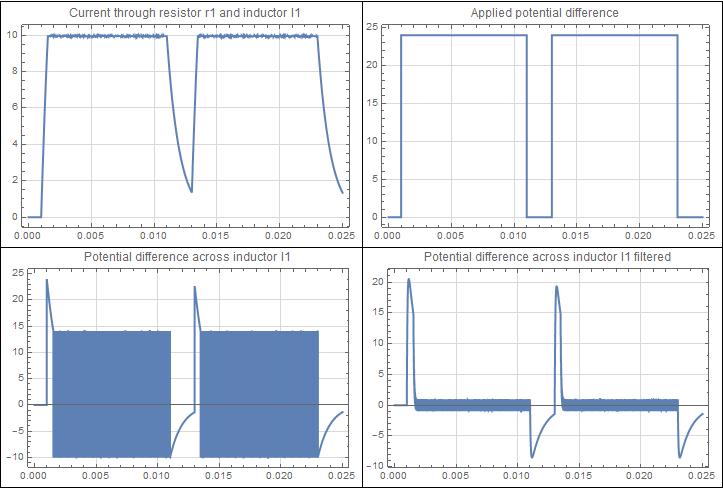
The results depend of the way the voltage source limits the current (slowly ? quickly ? is there a decoupling capacitor ?).

The following solution supposes that the source switches brutally from to 0V when I>10A and returns brutally to the normal value when I<9.9A.

The relevant code is :

• eq1 = k[t] v1[t] == (i[t]*r1 + l1*i'[t]); (* k[t] = 0 or 1 *)
• NDSolve[... eq1 ... WhenEvent[i[t]>10,k[t]->0],WhenEvent[i[t]<9.9,k[t]->1]]

The whole code :

  ClearAll["Global`*"]

(*inductance*) l1 = 0.001;
(*resistance*) r1 = 1;
(*pulsed voltage 1*) vUp = 24;
(*pulsed voltage 0*) vDown = 0;
(*voltage source definition*) 
v1[t_] := 
  Piecewise[{{vUp, 0.001 <= t <= 0.011}, {vUp, 0.013 <= t <= 0.023}}, 
   vDown];
(*ImageSize in plots*) imgSize = 350;
(*Model time*) time = 0.025;

eq1 = k[t]  v1[t] ==  (i[t]*r1 + l1*i'[t]); (* k[t] = 0 or 1 *)
eq2 = vfil[t] + 5. 10^-5 vfil'[t] == l1*i'[t]; (* just a filter to see the 
filtered voltage across the self *)

ic1 = i[0] == 0;

sol = NDSolveValue[{eq1, ic1, eq2, vfil[0]==0,k'[t]==1,k[0]==1,WhenEvent[i[t]>10,k[t]->  0 ],WhenEvent[i[t]<9.9,k[t]->  1 ]}, {i,vfil}, {t, 0, time}]

p1 = Plot[v1[t], {t, 0, time},
   PlotRange -> All,
   PlotPoints -> 200,
   AxesOrigin -> {0, 0},
   Frame -> True,
   GridLines -> Automatic,
   GridLinesStyle -> LightGray,
   PlotLabel -> "Applied potential difference",
   PlotStyle -> Thick,
   Exclusions -> 
    None (*for connection of piecewise function v1 in step up/down*),
   ImageSize -> imgSize
   ];

p2 = Plot[sol[[1]][t], {t, 0, time},
   PlotRange -> All,
   PlotPoints -> 200,
   AxesOrigin -> {0, 0},
   Frame -> True,
   GridLines -> Automatic,
   GridLinesStyle -> LightGray,
   PlotLabel -> "Current through resistor r1 and inductor l1",
   PlotStyle -> Thick,
   ImageSize -> imgSize
   ];

p3 = Plot[sol[[1]]'[t]*l1, {t, 0, time},
   PlotRange -> All,
   PlotPoints -> 300,
   AxesOrigin -> {0, 0},
   Frame -> True,
   GridLines -> Automatic,
   GridLinesStyle -> LightGray,
   PlotLabel -> "Potential difference across inductor l1",
   PlotStyle -> Thick,
   Exclusions -> None,
   ImageSize -> imgSize
   ];
   
 p4 = Plot[sol[[2]][t] , {t, 0, time},
   PlotRange -> All,
   PlotPoints -> 300,
   AxesOrigin -> {0, 0},
   Frame -> True,
   GridLines -> Automatic,
   GridLinesStyle -> LightGray,
   PlotLabel -> "Potential difference across inductor l1 filtered",
   PlotStyle -> Thick,
   Exclusions -> None,
   ImageSize -> imgSize
   ];

Grid[{{p2, p1}, {p3,p4}}, Frame -> True]