This is not an answer but a remark about the boundary conditions.

Let's look at the equation:

r1 = 10^(-6);
r2 = 95/10;
lambda = 1/10;
eqn = {r^2*D[D[a[r], r], r] == 
    a[r]*(a[r] - 1)*(a[r] - 2) - r^2*h[r]^2*(1 - a[r]), 
   D[r^2*D[h[r], r], r] == 
    2*h[r]*(1 - a[r])^2 + \[Lambda]*r^2*(h[r]^2 - 1)*h[r]};
bc = {a[r1] == 0, a[r2] == 1, h[r1] == 0, h[r2] == 1};
{teqn, tbc} = {eqn, bc} /. {a -> (#1^2*g[#1] &), h -> (#1*j[#1] &)};
teqn /. {g -> u, j -> v} // Expand;
{gsol, jsol} = 
  NDSolveValue[{teqn, tbc} /. \[Lambda] -> lambda, {g, j}, {r, r1, 
    r2}, Method -> {"ExplicitRungeKutta", "DifferenceOrder" -> 5}, 
   WorkingPrecision -> MachinePrecision];

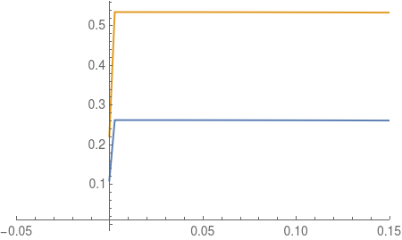
If we look at the plot:

Plot[{gsol[r], jsol[r]}, {r, r1, r2}, 
 PlotRange -> {{-0.05, 0.15}, All}]

We note a jump at the left hand side. The solver has trouble satisfying this BC (and the solver xzczd wrote has a similar problem).

The actual values:

{gsol[r] - 0, jsol[r] - 0} /. r -> r1
{gsol[r] - 1/90.25, jsol[r] - 1/9.5} /. r -> r2

{0.00147074, 1.38778*10^-16}
{-1.23805*10^-10, 2.58372*10^-11}

Do not quite match the requested bc at r1 for gsol.

If you were, just for fun (this is not the right thing to do), to replace the bcs in the following way:

{gsol2, jsol2} = 
  NDSolveValue[{teqn, {g[1/1000000] == gsol[0.001], 
      90.25` g[9.5`] == 1, j[1/1000000] == jsol[0.001], 
      9.5` j[9.5`] == 1}} /. \[Lambda] -> lambda, {g, j}, {r, r1, r2},
    Method -> {"ExplicitRungeKutta", "DifferenceOrder" -> 5}, 
   WorkingPrecision -> MachinePrecision];

You will note that the convergence is much quicker then with the above BCs. Where did you find these BCs. Are sure they make sense and are correct?