deleted 3 characters in body
Source Link
kglr
  • 400.5k
  • 18
  • 488
  • 929
data = RandomVariate[BinormalDistribution[.5], 200];
skdPDF = PDF[SmoothKernelDistribution[data]];

We defineDefine multivariate "quantiles" based on the height of the kernel density function. The function volume[z] gives the total probability of the set of points where density exceeds z:

volume[z_?NumericQ] := Quiet @ NIntegrate[skdPDF[{s, t}]Boole[skdPDF[{s, t}] >= z],
  {s, -∞, ∞}, {t, -∞, ∞}]

Find the density threshold levels corresponding to desired probability coverages (this is very slow):

{t99, t95, t68} = Quiet[FindRoot[volume[z] - # == 0, {z, 0, 1}]]& /@ {.99, .95, .68}

{{z -> 0.002508}, {z -> 0.008514}, {z -> 0.045498}}

SmoothDensityHistogram[data, MeshFunctions -> {skdPDF[{#, #2}] &}, 
  Mesh -> {{{z /. t99, Red}, {z /. t95, Green}, {z /. t68, Purple}}},
  MeshStyle -> Thick, PlotRange -> {{-4, 4}, {-4, 4}},
  Epilog -> {Black, PointSize[Medium], Point @ data}]

enter image description here

data = RandomVariate[BinormalDistribution[.5], 200];
skdPDF = PDF[SmoothKernelDistribution[data]];

We define multivariate "quantiles" based on the height of the density function. The function volume[z] gives the total probability of the set of points where density exceeds z:

volume[z_?NumericQ] := Quiet @ NIntegrate[skdPDF[{s, t}]Boole[skdPDF[{s, t}] >= z],
  {s, -∞, ∞}, {t, -∞, ∞}]

Find the density threshold levels corresponding to desired probability coverages (this is very slow):

{t99, t95, t68} = Quiet[FindRoot[volume[z] - # == 0, {z, 0, 1}]]& /@ {.99, .95, .68}

{{z -> 0.002508}, {z -> 0.008514}, {z -> 0.045498}}

SmoothDensityHistogram[data, MeshFunctions -> {skdPDF[{#, #2}] &}, 
  Mesh -> {{{z /. t99, Red}, {z /. t95, Green}, {z /. t68, Purple}}},
  MeshStyle -> Thick, PlotRange -> {{-4, 4}, {-4, 4}},
  Epilog -> {Black, PointSize[Medium], Point @ data}]
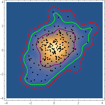
enter image description here

data = RandomVariate[BinormalDistribution[.5], 200];
skdPDF = PDF[SmoothKernelDistribution[data]];

Define multivariate "quantiles" based on the height of the kernel density function. The function volume[z] gives the total probability of the set of points where density exceeds z:

volume[z_?NumericQ] := Quiet @ NIntegrate[skdPDF[{s, t}]Boole[skdPDF[{s, t}] >= z],
  {s, -∞, ∞}, {t, -∞, ∞}]

Find the density threshold levels corresponding to desired probability coverages (this is very slow):

{t99, t95, t68} = Quiet[FindRoot[volume[z] - # == 0, {z, 0, 1}]]& /@ {.99, .95, .68}

{{z -> 0.002508}, {z -> 0.008514}, {z -> 0.045498}}

SmoothDensityHistogram[data, MeshFunctions -> {skdPDF[{#, #2}] &}, 
  Mesh -> {{{z /. t99, Red}, {z /. t95, Green}, {z /. t68, Purple}}},
  MeshStyle -> Thick, PlotRange -> {{-4, 4}, {-4, 4}},
  Epilog -> {Black, PointSize[Medium], Point @ data}]

enter image description here

added 266 characters in body
Source Link
kglr
  • 400.5k
  • 18
  • 488
  • 929
data = RandomVariate[BinormalDistribution[.5], 200];
skdPDF = PDF[SmoothKernelDistribution[data]];
 

We define multivariate "quantiles" based on the height of the density function. The function volume[z] gives the total probability of the set of points where density exceeds z:

volume[z_?NumericQ] := Quiet @ NIntegrate[skdPDF[{s, t}]Boole[skdPDF[{s, t}] >= z],
  {s, -Infinity, Infinity}, {t, -Infinity, Infinity}]
 

Find the density threshold levels corresponding to desired probability coverages (this is very slow):

{t99, t95, t68} = Quiet[FindRoot[volume[z] - # == 0, {z, 0, 1}]]& /@ {.99, .95, .68}

{{z -> 0.002508}, {z -> 0.008514}, {z -> 0.045498}}

 SmoothDensityHistogram[data, MeshFunctions -> {skdPDF[{#, #2}] &}, 
  Mesh -> {{{z /. t99, Red}, {z /. t95, Green}, {z /. t68, Purple}}},
  MeshStyle -> Thick, PlotRange -> {{-4, 4}, {-4, 4}},
  Epilog -> {Black, PointSize[Medium], Point @ data}]

enter image description here

data = RandomVariate[BinormalDistribution[.5], 200];
skdPDF = PDF[SmoothKernelDistribution[data]];
 
volume[z_?NumericQ]:= Quiet @ NIntegrate[skdPDF[{s,t}]Boole[skdPDF[{s,t}] >= z],
  {s, -Infinity, Infinity}, {t, -Infinity, Infinity}]
 
{t99, t95, t68} = Quiet[FindRoot[volume[z]- # == 0, {z, 0, 1}]]& /@ {.99, .95, .68}

{{z -> 0.002508}, {z -> 0.008514}, {z -> 0.045498}}

 SmoothDensityHistogram[data, MeshFunctions -> {skdPDF[{#, #2}] &}, 
  Mesh -> {{{z /. t99, Red}, {z /. t95, Green}, {z /. t68, Purple}}},
  MeshStyle -> Thick, PlotRange -> {{-4, 4}, {-4, 4}},
  Epilog -> {Black, PointSize[Medium], Point @ data}]

enter image description here

data = RandomVariate[BinormalDistribution[.5], 200];
skdPDF = PDF[SmoothKernelDistribution[data]];

We define multivariate "quantiles" based on the height of the density function. The function volume[z] gives the total probability of the set of points where density exceeds z:

volume[z_?NumericQ] := Quiet @ NIntegrate[skdPDF[{s, t}]Boole[skdPDF[{s, t}] >= z],
  {s, -, }, {t, -, }]

Find the density threshold levels corresponding to desired probability coverages (this is very slow):

{t99, t95, t68} = Quiet[FindRoot[volume[z] - # == 0, {z, 0, 1}]]& /@ {.99, .95, .68}

{{z -> 0.002508}, {z -> 0.008514}, {z -> 0.045498}}

SmoothDensityHistogram[data, MeshFunctions -> {skdPDF[{#, #2}] &}, 
  Mesh -> {{{z /. t99, Red}, {z /. t95, Green}, {z /. t68, Purple}}},
  MeshStyle -> Thick, PlotRange -> {{-4, 4}, {-4, 4}},
  Epilog -> {Black, PointSize[Medium], Point @ data}]

enter image description here

Source Link
kglr
  • 400.5k
  • 18
  • 488
  • 929

data = RandomVariate[BinormalDistribution[.5], 200];
skdPDF = PDF[SmoothKernelDistribution[data]];

volume[z_?NumericQ]:= Quiet @ NIntegrate[skdPDF[{s,t}]Boole[skdPDF[{s,t}] >= z],
  {s, -Infinity, Infinity}, {t, -Infinity, Infinity}]

{t99, t95, t68} = Quiet[FindRoot[volume[z]- # == 0, {z, 0, 1}]]& /@ {.99, .95, .68}

{{z -> 0.002508}, {z -> 0.008514}, {z -> 0.045498}}

 SmoothDensityHistogram[data, MeshFunctions -> {skdPDF[{#, #2}] &}, 
  Mesh -> {{{z /. t99, Red}, {z /. t95, Green}, {z /. t68, Purple}}},
  MeshStyle -> Thick, PlotRange -> {{-4, 4}, {-4, 4}},
  Epilog -> {Black, PointSize[Medium], Point @ data}]

enter image description here