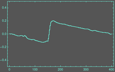
Doing this with basic image processing can be done. In comparison to the post you have linked, your situation is more complicated because you have a monochrome image with no option to separate colors. Additionally, your graph is surrounded by a frame.

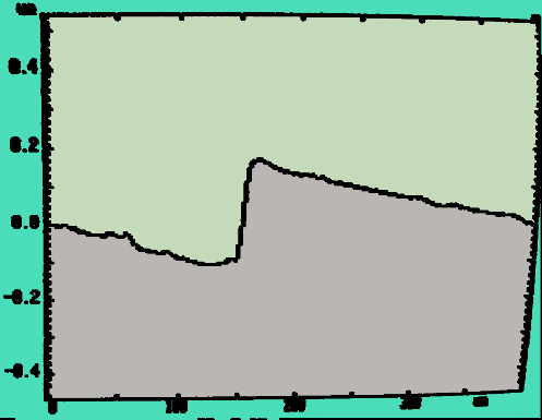
Let's assume we want to separate not the line but the area under or over the line that is inside the frame. This should be easy. Binarizing the negated image (and making the lines a bit thicker to close gaps):

bin = Erosion[ColorNegate[Binarize[img]], 1];
Colorize[MorphologicalComponents[bin]]

You can guess where this is going now. We separate the upper part and look at the vertical lengths of each line. There is a small transformation due to the round monitor but we ignore this for now:

masks = ComponentMeasurements[SelectComponents[bin, Large], "Mask"];
areas = MapAt[Image, masks, {All, 2}]

Now I'm just counting the number of ones in each column. Since the image is surrounded by a black margin, I'm cropping first. We use the upper part and therefore we need to negate the result to get an approximant of the line. Finally, we need to drop some elements from the start and the end to ensure we only have the data of the line

data = (-Count[1] /@ Transpose[ImageData[ImageCrop[1 /. areas], "Bit"]]);
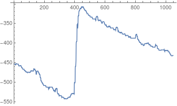
ListLinePlot[data[[18 ;; -18]]]

Now, we transform this into your coordinate system. To do so, we note that the start and the end hight of your graph are 0. Since we don't know the image transformation of the image we will choose a simple linear transformation that ensures that the first data-point and the last one will have a height of zero.

chopped = data[[18 ;; -18]];
lin[x_] := (chopped[[-1]] - chopped[[1]])/Length[chopped]*x

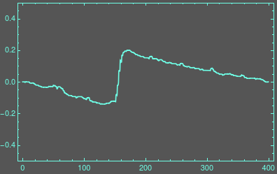
Now, we can reconstruct the original coordinate system and create an interpolating function that we can use to access it. We move the first data point to zero, apply our linear correction and in the end, we rescale the function so that the maximum peak is as 0.2 which looks about right from your image.

With[{d = Table[chopped[[i]] - chopped[[1]] - lin[i], {i, Length[chopped]}]},
  ip = ListInterpolation[d/Max[d]*.2, {{0, 400}}]
];

col = RGBColor[0.43, 1, .9];
Plot[ip[x], {x, 0, 400}, Axes -> False, Frame -> True, 
 PlotRange -> {Automatic, {-.5, .5}}, Background -> Darker[Gray], 
 FrameStyle -> col, PlotStyle -> col]

There are several errors with this approach. Most of all, we did not acknowledge the warping that your old curved monitor introduces. Second, the upper frame ticks in your image introduce small bumps in your curve because after all, we only count pixels.