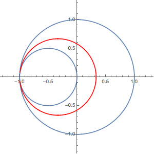
This is as close as you can get with machine precision:

F[-1 + $MachineEpsilon/2 + 0. I]
(*  -0.979196 + 0.165246 I  *)

One should think about how far the value is from -1 + 0 I, because it suggests closing the gap will be difficult. For instance, a delta-x of 10^-100 is almost acceptably close to -1:

N@F[-1 + 10.`100^-100]
(*  -0.999445 + 0.0271943 I  *)

In ParametricPlot, one can raise the WorkingPrecision, as well as MaxRecursion (to the max 15) and PlotPoints. (Increasing PlotPoints produces a marginally negligible improvement.)

For instance, this won't quite do it, because you'd probably need to raise PlotPoints to around 10^100:

ParametricPlot[{Limit[ReIm[F[xx + I*0]], xx -> x]}, {x, -1, 1}, 
 PlotRange -> {{-1.2, 1.2}, {-1.2, 1.2}}, MaxRecursion -> 15, 
 PlotPoints -> 200, PlotStyle -> Red, WorkingPrecision -> 50]

Using a substitution (x == Sin[t]) to get closer to ±1 helps:

Show[
 ParametricPlot[{Cos[x], Sin[x]}, {x, 0, 2 Pi}],
 ParametricPlot[{Cos[x]/2 - 1/2, Sin[x]/2}, {x, 0, 2 Pi}],
 ParametricPlot[{ReIm[F[Sin[t] + I*0]]}, {t, -Pi/2, Pi/2}, 
  MaxRecursion -> 15, PlotPoints -> 100, PlotStyle -> Red, 
  WorkingPrecision -> 50],
 ImageSize -> 300, PlotRange -> {{-1.2, 1.2}, {-1.2, 1.2}}]

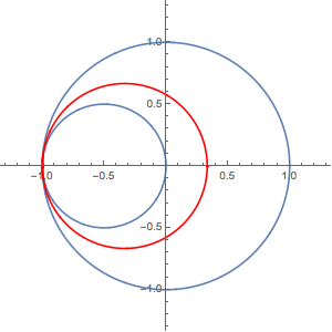
Here's the best I can do with producing a complete graph, but it's a bit slow:

ifn = NDSolveValue[{f'[x] == D[F[x + I*0], x], z'[x] == 1, z[0] == 0, 
   f[0] == F[0]}, f, {x, -1, 1}, PrecisionGoal -> 8, WorkingPrecision -> 1000]

Show[
 ParametricPlot[{Cos[x], Sin[x]}, {x, 0, 2 Pi}],
 ParametricPlot[{Cos[x]/2 - 1/2, Sin[x]/2}, {x, 0, 2 Pi}],
 ListLinePlot[ReIm@ifn["ValuesOnGrid"], PlotStyle -> Red, 
  PlotRange -> All],
 ImageSize -> 300]

It gets pretty close to -1:

ifn@ifn["Domain"] // N
(*  {{-0.999998 + 0.00263916 I, -0.999998 - 0.00263916 I}}  *)

BEWARE: Raising WorkingPrecision above 1000 in NDSolve above, which in theory would produce a better result, actually caused my kernel to crash.