added 369 characters in body
Source Link
bill s
  • 69.7k
  • 4
  • 103
  • 198

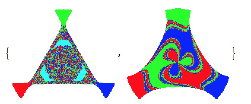
Since you presented the question in a visual manner, perhaps an image-based answer might be useful:

m1 = Import["E017.out", "Table"];
m2 = Import["E030.out", "Table"];
getColor[m_List, i_Integer] := 
  Module[{s = m[[i, 3]]}, 
   Which[s == -1, Black, s == 0, Cyan, s == 1, Green, s == 2, Red, 
    s == 3, Blue]];
data[m_] := 
  Table[{PointSize[0.005], getColor[m, i], 
    Point[{m[[i, 1]], m[[i, 2]]}]}, {i, 1, Length[m]}];
{S1 = Graphics[data[m1]], S2 = Graphics[data[m2]]}

enter image description here

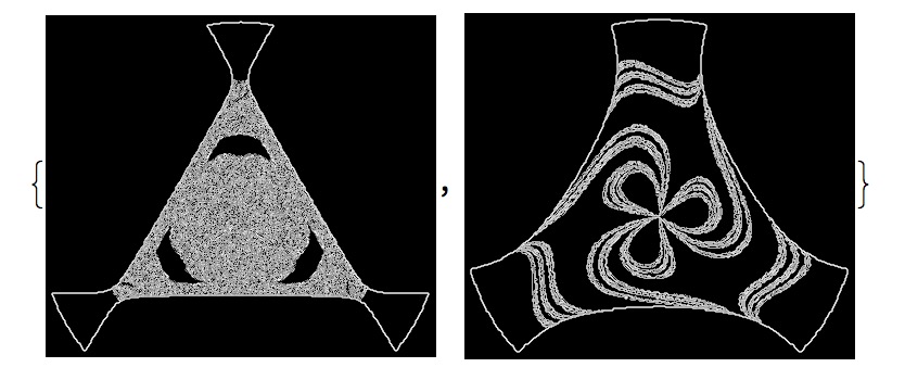
Taking the gradient of the images yields images with white where there are lots of changes and black in regions that are relatively constant.

{f1 = GradientFilter[Image[S1], 1], f2 = GradientFilter[Image[S2], 1]}

enter image description here

Now counting the white areas in the two filtered images gives a measure of how much change there is in each image.

{Total[ImageData[f1], 2], Total[ImageData[f2], 2]}
{14020.4, 10960.1}

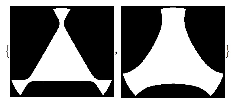
Since the quantity of interest is the percentage, we can create binary masks:

{mask1, mask2} = {Sign[ImageData[ColorNegate[ColorConvert[Image[S1], "Grayscale"]]]], 
    Sign[ImageData[ColorNegate[ColorConvert[Image[S2], "Grayscale"]]]]};
Image /@ {mask1, mask2}

enter image description here

Now we can calculate

{Total[ImageData[f1],2], Total[ImageData[f2],2]}/{Total[mask1,2], Total[mask2,2]}
{0.478201, 0.225147}

which shows that about 48% of the first one and 22% of the second are in regions where the behavior of the system is unpredictable.

Of course, one could substitute other filters: StandardDeviationFilter might make more statistical sense.

Since you presented the question in a visual manner, perhaps an image-based answer might be useful:

m1 = Import["E017.out", "Table"];
m2 = Import["E030.out", "Table"];
getColor[m_List, i_Integer] := 
  Module[{s = m[[i, 3]]}, 
   Which[s == -1, Black, s == 0, Cyan, s == 1, Green, s == 2, Red, 
    s == 3, Blue]];
data[m_] := 
  Table[{PointSize[0.005], getColor[m, i], 
    Point[{m[[i, 1]], m[[i, 2]]}]}, {i, 1, Length[m]}];
{S1 = Graphics[data[m1]], S2 = Graphics[data[m2]]}

enter image description here

Taking the gradient of the images yields images with white where there are lots of changes and black in regions that are relatively constant.

{f1 = GradientFilter[Image[S1], 1], f2 = GradientFilter[Image[S2], 1]}

enter image description here

Now counting the white areas in the two filtered images gives a measure of how much change there is in each image.

{Total[ImageData[f1], 2], Total[ImageData[f2], 2]}
{14020.4, 10960.1}

Since the quantity of interest is the percentage, we can create binary masks:

{mask1, mask2} = {Sign[ImageData[ColorNegate[ColorConvert[Image[S1], "Grayscale"]]]], 
    Sign[ImageData[ColorNegate[ColorConvert[Image[S2], "Grayscale"]]]]};
Image /@ {mask1, mask2}

Of course, one could substitute other filters: StandardDeviationFilter might make more statistical sense.
Since you presented the question in a visual manner, perhaps an image-based answer might be useful:

m1 = Import["E017.out", "Table"];
m2 = Import["E030.out", "Table"];
getColor[m_List, i_Integer] := 
  Module[{s = m[[i, 3]]}, 
   Which[s == -1, Black, s == 0, Cyan, s == 1, Green, s == 2, Red, 
    s == 3, Blue]];
data[m_] := 
  Table[{PointSize[0.005], getColor[m, i], 
    Point[{m[[i, 1]], m[[i, 2]]}]}, {i, 1, Length[m]}];
{S1 = Graphics[data[m1]], S2 = Graphics[data[m2]]}

enter image description here

Taking the gradient of the images yields images with white where there are lots of changes and black in regions that are relatively constant.

{f1 = GradientFilter[Image[S1], 1], f2 = GradientFilter[Image[S2], 1]}

enter image description here

Now counting the white areas in the two filtered images gives a measure of how much change there is in each image.

{Total[ImageData[f1], 2], Total[ImageData[f2], 2]}
{14020.4, 10960.1}

Since the quantity of interest is the percentage, we can create binary masks:

{mask1, mask2} = {Sign[ImageData[ColorNegate[ColorConvert[Image[S1], "Grayscale"]]]], 
    Sign[ImageData[ColorNegate[ColorConvert[Image[S2], "Grayscale"]]]]};
Image /@ {mask1, mask2}

enter image description here

Now we can calculate

{Total[ImageData[f1],2], Total[ImageData[f2],2]}/{Total[mask1,2], Total[mask2,2]}
{0.478201, 0.225147}

which shows that about 48% of the first one and 22% of the second are in regions where the behavior of the system is unpredictable.

Of course, one could substitute other filters: StandardDeviationFilter might make more statistical sense.
added 284 characters in body
Source Link
bill s
  • 69.7k
  • 4
  • 103
  • 198

Since you presented the question in a visual manner, perhaps an image-based answer might be useful:

m1 = Import["E017.out", "Table"];
m2 = Import["E030.out", "Table"];
getColor[m_List, i_Integer] := 
  Module[{s = m[[i, 3]]}, 
   Which[s == -1, Black, s == 0, Cyan, s == 1, Green, s == 2, Red, 
    s == 3, Blue]];
data[m_] := 
  Table[{PointSize[0.005], getColor[m, i], 
    Point[{m[[i, 1]], m[[i, 2]]}]}, {i, 1, Length[m]}];
{S1 = Graphics[data[m1]], S2 = Graphics[data[m2]]}

enter image description here

Taking the gradient of the images yields images with white where there are lots of changes and black in regions that are relatively constant.

{f1 = GradientFilter[Image[S1], 1], f2 = GradientFilter[Image[S2], 1]}

enter image description here

Now counting the white areas in the two filtered images gives a measure of how much change there is in each image.

{Total[ImageData[f1], 2], Total[ImageData[f2], 2]}
{14020.4, 10960.1}

Since the quantity of interest is the percentage, we can create binary masks:

{mask1, mask2} = {Sign[ImageData[ColorNegate[ColorConvert[Image[S1], "Grayscale"]]]], 
    Sign[ImageData[ColorNegate[ColorConvert[Image[S2], "Grayscale"]]]]};
Image /@ {mask1, mask2}

Of course, one could substitute other filters: StandardDeviationFilter might make more statistical sense.

Since you presented the question in a visual manner, perhaps an image-based answer might be useful:

m1 = Import["E017.out", "Table"];
m2 = Import["E030.out", "Table"];
getColor[m_List, i_Integer] := 
  Module[{s = m[[i, 3]]}, 
   Which[s == -1, Black, s == 0, Cyan, s == 1, Green, s == 2, Red, 
    s == 3, Blue]];
data[m_] := 
  Table[{PointSize[0.005], getColor[m, i], 
    Point[{m[[i, 1]], m[[i, 2]]}]}, {i, 1, Length[m]}];
{S1 = Graphics[data[m1]], S2 = Graphics[data[m2]]}

enter image description here

Taking the gradient of the images yields images with white where there are lots of changes and black in regions that are relatively constant.

{f1 = GradientFilter[Image[S1], 1], f2 = GradientFilter[Image[S2], 1]}

enter image description here

Now counting the white areas in the two filtered images gives a measure of how much change there is in each image.

{Total[ImageData[f1], 2], Total[ImageData[f2], 2]}
{14020.4, 10960.1}

Since the quantity of interest is the percentage, we can create binary masks:

{mask1, mask2} = {Sign[ImageData[ColorNegate[ColorConvert[Image[S1], "Grayscale"]]]], 
    Sign[ImageData[ColorNegate[ColorConvert[Image[S2], "Grayscale"]]]]};
Image /@ {mask1, mask2}

Of course, one could substitute other filters: StandardDeviationFilter might make more statistical sense.

Source Link
bill s
  • 69.7k
  • 4
  • 103
  • 198

Since you presented the question in a visual manner, perhaps an image-based answer might be useful:

m1 = Import["E017.out", "Table"];
m2 = Import["E030.out", "Table"];
getColor[m_List, i_Integer] := 
  Module[{s = m[[i, 3]]}, 
   Which[s == -1, Black, s == 0, Cyan, s == 1, Green, s == 2, Red, 
    s == 3, Blue]];
data[m_] := 
  Table[{PointSize[0.005], getColor[m, i], 
    Point[{m[[i, 1]], m[[i, 2]]}]}, {i, 1, Length[m]}];
{S1 = Graphics[data[m1]], S2 = Graphics[data[m2]]}

enter image description here

Taking the gradient of the images yields images with white where there are lots of changes and black in regions that are relatively constant.

{f1 = GradientFilter[Image[S1], 1], f2 = GradientFilter[Image[S2], 1]}

enter image description here

Now counting the white areas in the two filtered images gives a measure of how much change there is in each image.

{Total[ImageData[f1], 2], Total[ImageData[f2], 2]}
{14020.4, 10960.1}

Of course, one could substitute other filters: StandardDeviationFilter might make more statistical sense.