replaced http://mathematica.stackexchange.com/ with https://mathematica.stackexchange.com/
Source Link

Credit goes to @m_goldberg for his ideaidea.

The PDE in question cannot be handle directly by NDSolve. So we need to specify a Method. For this, I used MethodOfLines.

sol = NDSolve[{D[f[x, v, t], t] ==v*D[f[x, v, t], x] + D[f[x, v, t], v, v], 
   f[x, v, 0] == Exp[(-v^2 - x^2)/(2*0.001^2)]/(0.001*Sqrt[2 Pi]), 
   f[x, -100, t] == 0, f[x, 100, t] == 0, f[100, v, t] == 0}, 
  f, {v, -100.0, 100.0}, {t, 0.0, 50.0}, {x, -100.0, 100.0}, 
  Method -> {"MethodOfLines","SpatialDiscretization" -> {"TensorProductGrid", 
      "MinPoints" -> {30, 30}}, "TemporalVariable" -> t}];

Now extracting the interpolating function for external use,

{fF} = sol[[1, All, 2]];
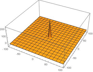
Plot3D[fF[x, v, 1], {x, -100.0, 100.0}, {v, -100.0, 100.0}, PlotRange -> Full]

enter image description here

Integrating the interpolating function,

Block[{x, t}, q[x_, t_] = Integrate[fF[x, v, t], {v, -100, 100}];]
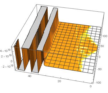
Plot3D[q[x, t], {x, -100.0, 100.0}, {t, 0, 50}, PlotPoints -> 30]

enter image description here

The above plot doesn't make any sense to me.

Credit goes to @m_goldberg for his idea.

The PDE in question cannot be handle directly by NDSolve. So we need to specify a Method. For this, I used MethodOfLines.

sol = NDSolve[{D[f[x, v, t], t] ==v*D[f[x, v, t], x] + D[f[x, v, t], v, v], 
   f[x, v, 0] == Exp[(-v^2 - x^2)/(2*0.001^2)]/(0.001*Sqrt[2 Pi]), 
   f[x, -100, t] == 0, f[x, 100, t] == 0, f[100, v, t] == 0}, 
  f, {v, -100.0, 100.0}, {t, 0.0, 50.0}, {x, -100.0, 100.0}, 
  Method -> {"MethodOfLines","SpatialDiscretization" -> {"TensorProductGrid", 
      "MinPoints" -> {30, 30}}, "TemporalVariable" -> t}];

Now extracting the interpolating function for external use,

{fF} = sol[[1, All, 2]];
Plot3D[fF[x, v, 1], {x, -100.0, 100.0}, {v, -100.0, 100.0}, PlotRange -> Full]

enter image description here

Integrating the interpolating function,

Block[{x, t}, q[x_, t_] = Integrate[fF[x, v, t], {v, -100, 100}];]
Plot3D[q[x, t], {x, -100.0, 100.0}, {t, 0, 50}, PlotPoints -> 30]

enter image description here

The above plot doesn't make any sense to me.
Credit goes to @m_goldberg for his idea.

The PDE in question cannot be handle directly by NDSolve. So we need to specify a Method. For this, I used MethodOfLines.

sol = NDSolve[{D[f[x, v, t], t] ==v*D[f[x, v, t], x] + D[f[x, v, t], v, v], 
   f[x, v, 0] == Exp[(-v^2 - x^2)/(2*0.001^2)]/(0.001*Sqrt[2 Pi]), 
   f[x, -100, t] == 0, f[x, 100, t] == 0, f[100, v, t] == 0}, 
  f, {v, -100.0, 100.0}, {t, 0.0, 50.0}, {x, -100.0, 100.0}, 
  Method -> {"MethodOfLines","SpatialDiscretization" -> {"TensorProductGrid", 
      "MinPoints" -> {30, 30}}, "TemporalVariable" -> t}];

Now extracting the interpolating function for external use,

{fF} = sol[[1, All, 2]];
Plot3D[fF[x, v, 1], {x, -100.0, 100.0}, {v, -100.0, 100.0}, PlotRange -> Full]

enter image description here

Integrating the interpolating function,

Block[{x, t}, q[x_, t_] = Integrate[fF[x, v, t], {v, -100, 100}];]
Plot3D[q[x, t], {x, -100.0, 100.0}, {t, 0, 50}, PlotPoints -> 30]

enter image description here

The above plot doesn't make any sense to me.
Source Link
zhk
  • 12k
  • 1
  • 23
  • 39

Credit goes to @m_goldberg for his idea.

The PDE in question cannot be handle directly by NDSolve. So we need to specify a Method. For this, I used MethodOfLines.

sol = NDSolve[{D[f[x, v, t], t] ==v*D[f[x, v, t], x] + D[f[x, v, t], v, v], 
   f[x, v, 0] == Exp[(-v^2 - x^2)/(2*0.001^2)]/(0.001*Sqrt[2 Pi]), 
   f[x, -100, t] == 0, f[x, 100, t] == 0, f[100, v, t] == 0}, 
  f, {v, -100.0, 100.0}, {t, 0.0, 50.0}, {x, -100.0, 100.0}, 
  Method -> {"MethodOfLines","SpatialDiscretization" -> {"TensorProductGrid", 
      "MinPoints" -> {30, 30}}, "TemporalVariable" -> t}];

Now extracting the interpolating function for external use,

{fF} = sol[[1, All, 2]];
Plot3D[fF[x, v, 1], {x, -100.0, 100.0}, {v, -100.0, 100.0}, PlotRange -> Full]

enter image description here

Integrating the interpolating function,

Block[{x, t}, q[x_, t_] = Integrate[fF[x, v, t], {v, -100, 100}];]
Plot3D[q[x, t], {x, -100.0, 100.0}, {t, 0, 50}, PlotPoints -> 30]

enter image description here

The above plot doesn't make any sense to me.