Since your code, doesn't work, I wrote my own simplified version:
g[x_,t_] = NDSolveValue[{
  D[f[x, t], t] == D[f[x, t], {x, 2}]
  , f[x, 0] == Sin[x]
  , f[0, t] == 0, f[π, t] == 0
 }
 , f[x, t]
 , {x, 0, 1}, {t, 0, 5}];
Note that I am using NDSolveValue to spit out the function automatically. You can then directly integrate the function:
integratedG[t_] = Integrate[g[x, t], {x, 0, 1}];
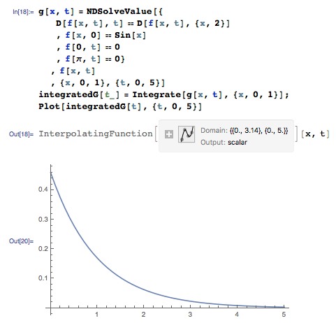
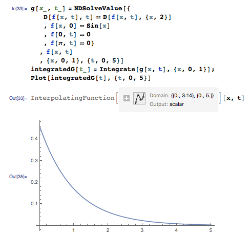
and the result is another interpolating function that you can then plot:
. The reason that this works is that behind the scenes, an InterpolatingFunction consists of a bunch of polynomials, which are obviously easy to analytically integrate, and Mathematica does that automatically.
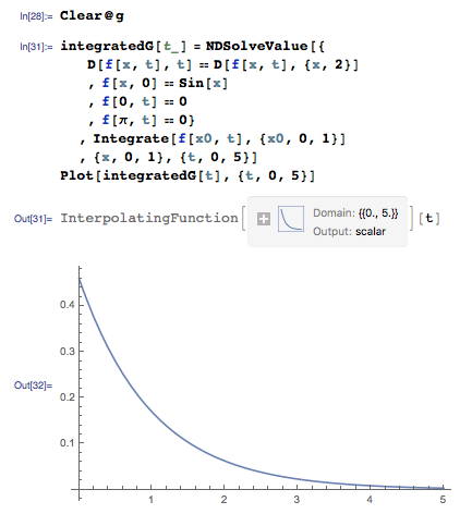
Alternatively, if you don't need the function itself, you can build this directly into the call to NDSolveValue:
integratedG[t_] = NDSolveValue[{
   D[f[x, t], t] == D[f[x, t], {x, 2}]
   , f[x, 0] == Sin[x]
   , f[0, t] == 0
   , f[π, t] == 0}
  , Integrate[f[x0, t], {x0, 0, 1}]
  , {x, 0, 1}, {t, 0, 5}];
To wit:
or


