Bounty Ended with 100 reputation awarded by user21
added direct response to OP's code
Source Link

EDIT: correction of your boundary conditions

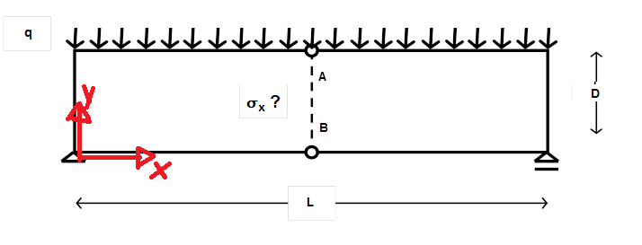
Hey Gonza_! In your code, you wanted to treat the mechanical problem as follows.

enter image description here

You only had a slight syntax error in your boundary conditions

(*Wrong*)
bcwrong = {
   DirichletCondition[v[x, y] == 0, {x == 0, y == 0}]
   , DirichletCondition[u[x, y] == 0, {x == 0, y == 0}]
   , DirichletCondition[v[x, y] == 0, {x == L, y == 0}]
   };
(*Correct*)
bccorrect = {
   DirichletCondition[{u[x, y] == 0, v[x, y] == 0}, x == 0 && y == 0]
   , DirichletCondition[v[x, y] == 0, x == L && y == 0]
   };

The difference is that the bcwrong impose a vanishing displacement field at every point with x==0 and at every point with y==0. The correct syntax is given in bccorrect. Working code:

Needs["NDSolve`FEM`"];
(*Geometry*)
L = 2;
h1 = 1/2;
Reg1 = Rectangle[{0, 0}, {L, h1}];
Mesh1 = ToElementMesh[Reg1, MeshQualityGoal -> 0];
(*Forces*)
q = 6000;
(*Material properties*)
Propiedades = {Y -> 205940000000, \[Nu] -> 30/100};
(*2D Hooke's law*)
hl = {
   \[Sigma]x[x, y] == 
    Y/(1 - \[Nu]^2) (D[u[x, y], x] + \[Nu] D[v[x, y], y])
   , \[Sigma]y[x, y] == 
    Y/(1 - \[Nu]^2) (D[v[x, y], y] + \[Nu] D[u[x, y], x])
   , \[Sigma]xy[x, 
     y] == (Y*\[Nu])/(1 - \[Nu]^2) (D[u[x, y], x] + D[v[x, y], y])
   };
(*Equations*)
PS = {Inactive[
      Div][{{0, -((Y \[Nu])/(1 - \[Nu]^2))}, {-((Y (1 - \[Nu]))/(2 (1 \
- \[Nu]^2))), 0}}.Inactive[Grad][v[x, y], {x, y}], {x, y}] + 
    Inactive[
      Div][{{-(Y/(1 - \[Nu]^2)), 
        0}, {0, -((Y (1 - \[Nu]))/(2 (1 - \[Nu]^2)))}}.Inactive[Grad][
       u[x, y], {x, y}], {x, y}], 
   Inactive[
      Div][{{0, -((Y (1 - \[Nu]))/(2 (1 - \[Nu]^2)))}, {-((Y \
\[Nu])/(1 - \[Nu]^2)), 0}}.Inactive[Grad][u[x, y], {x, y}], {x, y}] + 
    Inactive[
      Div][{{-((Y (1 - \[Nu]))/(2 (1 - \[Nu]^2))), 
        0}, {0, -(Y/(1 - \[Nu]^2))}}.Inactive[Grad][
       v[x, y], {x, y}], {x, y}]};
(*BCs*)
(*Neumann*)
bcN = {0, NeumannValue[-q, y == h1]};
(*Wrong*)
bcwrong = {
   DirichletCondition[v[x, y] == 0, {x == 0, y == 0}]
   , DirichletCondition[u[x, y] == 0, {x == 0, y == 0}]
   , DirichletCondition[v[x, y] == 0, {x == L, y == 0}]
   };
(*Correct*)
bccorrect = {
   DirichletCondition[{u[x, y] == 0, v[x, y] == 0}, x == 0 && y == 0]
   , DirichletCondition[v[x, y] == 0, x == L && y == 0]
   };
(*FEM-solution*)
{u1, v1, \[Sigma]x1, \[Sigma]y1, \[Tau]xy1} = 
  NDSolveValue[{PS == bcN, hl, bccorrect} /. Propiedades, {u, 
    v, \[Sigma]x, \[Sigma]y, \[Sigma]xy}
   , Element[{x, y}, Mesh1]];
(*Deformation*)
DMesh1 = ElementMeshDeformation[Mesh1, {u1, v1}, 
   "ScalingFactor" -> 6*10^4];
Show[{Mesh1[
   "Wireframe"[
    "ElementMeshDirective" -> Directive[EdgeForm[Gray], FaceForm[]]]],
   DMesh1[
   "Wireframe"[
    "ElementMeshDirective" -> 
     Directive[EdgeForm[RGBColor[0, 0.3, 0.8]], FaceForm[]]]]}, 
 ImageSize -> 300]
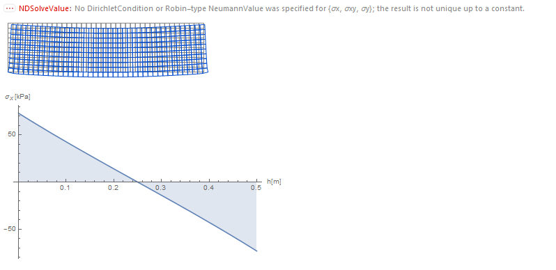
(*Normal stress at x=L/2 depending on y*)
Plot[\[Sigma]x1[L/2, y]/1000, {y, 0, h1}, Filling -> Axis, 
 AxesLabel -> {"h[m]", 
   "\!\(\*SubscriptBox[\(\[Sigma]\), \(x\)]\)[kPa]"}, 
 ImageSize -> 400]

enter image description here


General 3D theory

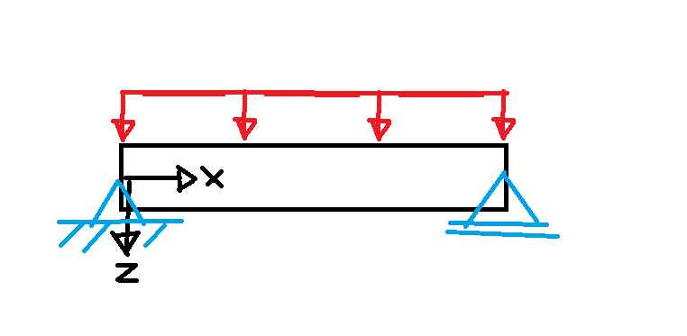
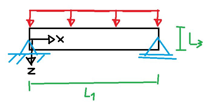
updated picture of mechanical problem
Source Link

You can get the stress distribution at any point with the full 3D Hooke's law $\sigma_{ij} = C_{ijkl} u_{k,l}$ (FEM solution as red points) (remark: you dont need to symmetrize the displacement grandient in my code in order to obtain the infinitesimal strain, since the stiffness $C_{ijkl}$ I used symmetrizes automatically the mapped tensor). Let's get $\sigma_{xx} = \sigma_{11}$

uv[x_, y_, z_] := {usol[x, y, z], vsol[x, y, z], wsol[x, y, z]}
eps[xs_, ys_, zs_] := 
 D[uv[x, y, z], {{x, y, z}, 1}] /. {x -> xs, y -> ys, z -> zs}
(*linear map of second order tensor B over fourth-order tensor A*)
lm[A_, B_] := TensorContract[TensorProduct[A, B], {{3, 5}, {4, 6}}]
(*Get Cauchy stress sigma_xx = sigma[[1,1]], at x==L1x=L1/2 depending on z with 3D Hooke's law*)
sigloc = lm[Ciso, eps[L1/2, 0, z]][[1, 1]];
siglocdata = Table[{zi, sigloc /. z -> zi}, {zi, -L3/2, L3/2, L3/10}];
Plot[sig /. x -> L1/2, {z, -L3/2, L3/2}, 
 AxesLabel -> {"z", "\[Sigma](x=L1/2,z)"}, 
 Epilog -> {PointSize -> Medium, Red, Point@siglocdata}]

You can get the stress distribution at any point with the full 3D Hooke's law $\sigma_{ij} = C_{ijkl} u_{k,l}$ (FEM solution as red points) (remark: you dont need to symmetrize the displacement grandient in my code in order to obtain the infinitesimal strain, since the stiffness $C_{ijkl}$ I used symmetrizes automatically the mapped tensor)

uv[x_, y_, z_] := {usol[x, y, z], vsol[x, y, z], wsol[x, y, z]}
eps[xs_, ys_, zs_] := 
 D[uv[x, y, z], {{x, y, z}, 1}] /. {x -> xs, y -> ys, z -> zs}
(*linear map of second order tensor B over fourth-order tensor A*)
lm[A_, B_] := TensorContract[TensorProduct[A, B], {{3, 5}, {4, 6}}]
(*Get Cauchy stress at x==L1/2 depending on z with 3D Hooke's law*)
sigloc = lm[Ciso, eps[L1/2, 0, z]][[1, 1]];
siglocdata = Table[{zi, sigloc /. z -> zi}, {zi, -L3/2, L3/2, L3/10}];
Plot[sig /. x -> L1/2, {z, -L3/2, L3/2}, 
 AxesLabel -> {"z", "\[Sigma](x=L1/2,z)"}, 
 Epilog -> {PointSize -> Medium, Red, Point@siglocdata}]

You can get the stress distribution at any point with the full 3D Hooke's law $\sigma_{ij} = C_{ijkl} u_{k,l}$ (FEM solution as red points) (remark: you dont need to symmetrize the displacement grandient in my code in order to obtain the infinitesimal strain, since the stiffness $C_{ijkl}$ I used symmetrizes automatically the mapped tensor). Let's get $\sigma_{xx} = \sigma_{11}$

uv[x_, y_, z_] := {usol[x, y, z], vsol[x, y, z], wsol[x, y, z]}
eps[xs_, ys_, zs_] := 
 D[uv[x, y, z], {{x, y, z}, 1}] /. {x -> xs, y -> ys, z -> zs}
(*linear map of second order tensor B over fourth-order tensor A*)
lm[A_, B_] := TensorContract[TensorProduct[A, B], {{3, 5}, {4, 6}}]
(*Get Cauchy stress sigma_xx = sigma[[1,1]], at x=L1/2 depending on z with 3D Hooke's law*)
sigloc = lm[Ciso, eps[L1/2, 0, z]][[1, 1]];
siglocdata = Table[{zi, sigloc /. z -> zi}, {zi, -L3/2, L3/2, L3/10}];
Plot[sig /. x -> L1/2, {z, -L3/2, L3/2}, 
 AxesLabel -> {"z", "\[Sigma](x=L1/2,z)"}, 
 Epilog -> {PointSize -> Medium, Red, Point@siglocdata}]
updated picture of mechanical problem
Source Link

enter image description hereenter image description here

enter image description here

enter image description here

remark to Hooke's law in code
Source Link
Loading
picture of mechanical problem added
Source Link
Loading
Source Link
Loading