One can still speed up your code a lot
rp3[A_, B_] := Module[{a,c},
  a = Transpose[A];
  c = B;
  Do[c = Transpose[c.a, {2, 3, 4, 1}], {i, 4}];
  c
  ]
Now timing subroutine:
test[n_] := Module[{t0, t1, nrm, A, B,c0,c1},
  A = RandomInteger[{-10, 10}, {n, n}];
  B = RandomInteger[{-10, 10}, {n, n, n, n}];
  t0 = Timing[c0 = rp2[A, B];] // First;
  t1 = Timing[c10Timing[c1 = rp3[A, B];] // First;
  nrm = Norm[Flatten[c10Norm[Flatten[c1 - c0]];
  {n, t0, t1, nrm}
  ]
Now results:
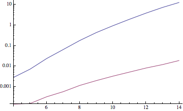
p = Table[test[n], {n, 4, 14}]
(*{{4, 0.002887, 0.000146, 0}, {5, 0.007295, 0.000156, 0}, {6, 0.023915,
   0.000331, 0}, {7, 0.065420, 0.000586, 0}, {8, 0.180312, 0.001182,
  0}, {9, 0.437847, 0.002028, 0}, {10, 0.942596, 0.003337, 0}, {11,
  1.941590, 0.005264, 0}, {12, 3.863945, 0.008290, 0}, {13, 7.321387,
  0.012194, 0}, {14, 12.766735, 0.019249, 0}}*)
Now plots
ListLogPlot[{p[[All, 1 ;; 2]], p[[All, 1 ;; 3 ;; 2]]}, Joined -> True]
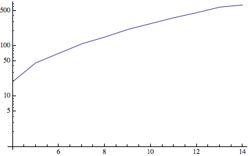
speedup = Transpose[{p[[All, 1]], p[[All, 2]]/p[[All, 3]]}]
(*{{4, 20.}, {5, 47.}, {6, 72.}, {7, 112.}, {8, 153.}, {9, 216.}, {10,
  282.5}, {11, 368.8}, {12, 466.1}, {13, 600.4}, {14, 663.2}}*)
ListLogPlot[speedup, Joined -> True]
Comparison of run-times
Speed up
For sizes in the range of 4 to 14 we have a speedup in the range of 20 to 663 !
Explanation
Matrix-matrix multiplication is much faster than a set of corresponding matrix-vector multiplications!


